This is a summary of chapter 3 of the Introduction to Statistical Learning textbook. I’ve written a 10-part guide that covers the entire book. The guide can be read at my website, or here at Hashnode. Subscribe to stay up to date on my latest Data Science & Engineering guides!

Simple Linear Regression

Simple linear regression assumes a linear relationship between the predictor (X) and the response (Y). A simple linear regression model takes the following form:

• y-hat — represents the predicted value
• β₀— represents a coefficient known as the intercept
• β₁ — represents a coefficient known as the slope
• X— represents the value of the predictor

For example, we could build a simple linear regression model from the following statistician salary dataset:

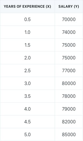
The simple linear regression model could be written as follows:

Least Squares Criteria

The best estimates for the coefficients (β₀, β₁) are obtained by finding the regression line that fits the training dataset points as closely as possible. This line can be obtained by minimizing the least squares criteria.

What does it mean to minimize the least squares criteria? Let’s use the example of the regression model for the statistician salaries.

The difference between the actual salary value and the predicted salary is known as the residual (e). The residual sum of squares (RSS) is defined as:

The least squares criteria chooses the β coefficient values that minimize the RSS.

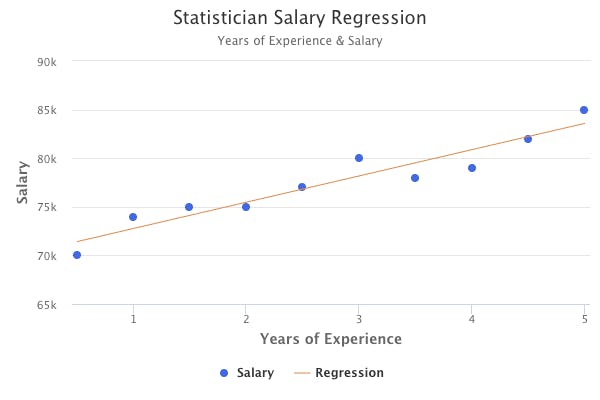
For our statistician salary dataset, the linear regression model determined through the least squares criteria is as follows:

• β₀ is $70,545
• β₁ is $2,576

This final regression model can be visualized by the orange line below:

Interpretation of β Coefficients​

How do we interpret the coefficients of a simple linear regression model in plain English? In general, we say that:

• If the predictor (X) were 0, the prediction (Y) would be β₀, on average.
• For every one increase in the predictor, the prediction changes by β₁, on average.

Using the example of the final statistician salary regression model, we would conclude that:

• If a statistician had 0 years of experience, he/she would have an entry-level salary of $70,545, on average.
• For every one additional year of experience that a statistician has, his/her salary increases by $2,576, on average.

True Population Regression vs Least Squares Regression

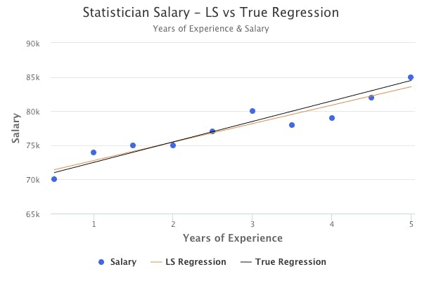
The true population regression line represents the “true” relationship between X and Y. However, we never know the true relationship, so we use least squares regression to estimate it with the data that we have available.

For example, assume that the true population regression line for statistician salaries was represented by the black line below. The least squares regression line, represented by the orange line, is close to the true population regression line, but not exactly the same.

So, how do we estimate how accurate the least squares regression line is as an estimate of the true population regression line?

We compute the standard error of the coefficients and determine the confidence interval.

The standard error is a measure of the accuracy of an estimate. Knowing how to mathematically calculate the standard error is not important, as programs like R will determine them easily.

Standard errors are used to compute confidence intervals, which provide an estimate of how accurate the least squares regression line is.

The most commonly used confidence interval is the 95% confidence interval.

The confidence interval is generally interpreted as follows:

• There is a 95% probability that the interval contains the true population value of the coefficient.

For example, for the statistician salary regression model, the confidence intervals are as follows:

• β₀ = [67852,72281]
• β₁ = [1989,3417]

In the context of the statistician salaries, these confidence intervals are interpreted as follows:

• In the absence of any years of experience, the salary of an entry-level statistician will fall between $67,852 and $72,281.
• For each one additional year of experience, a statistician’s salary will increase between $1,989 and $3,417.

Hypothesis Testing

So, how do we determine whether or not there truly is a relationship between X and Y? In other words, how do we know that X is actually a good predictor for Y?

We use the standard errors to perform hypothesis tests on the coefficients.

The most common hypothesis test involves testing the null hypothesis versus the alternative hypothesis:

• Null Hypothesis: No relationship between X and Y
• Alternative Hypothesis: Some relationship between X and Y

t-statistic and p-value

So, how do we determine if β₁ is non-zero? We use the estimated value of the coefficient and its standard error to determine the t-statistic:

The t-statistic measures the number of standard deviations that β₁ is away from 0.

The t-statistic allows us to determine something known as the p-value, which ultimately helps determine whether or not the coefficient is non-zero.

The p-value indicates how likely it is to observe a meaningful association between X and Y by some bizarre random error or chance, as opposed to there being a true relationship between X and Y.

Typically, we want p-values less than 5% or 1% to reject the null hypothesis. In other words, rejecting the null hypothesis means that we are declaring that some relationship exists between X and Y.

Assessing Model Accuracy

There are 2 main assessments for how well a model fits the data: RSE and R².

Residual Standard Error (RSE)

The RSE is a measure of the standard deviation of the random error term (ϵ).

In other words, it is the average amount that the actual response will deviate from the true regression line. It is a measure of the lack of fit of a model.

The value of RSE and whether or not it is acceptable will depend on the context of the problem.

R-Squared (R²)

R² measures the proportion of variability in Y that can be explained by using X. It is a proportion that is calculated as follows:

TSS is a measure of variability that is already inherent in the response variable before regression is performed.

RSS is a measure of variability in the response variable after regression is performed.

The final statistician salary regression model has an R² of 0.90, meaning that 90% of the variability in the salaries of statisticians is explained by using years of experience as a predictor.

Multiple Linear Regression

Simple linear regression is useful for prediction if there is only one predictor. But what if we had multiple predictors? Multiple linear regression allows for multiple predictors, and takes the following form:

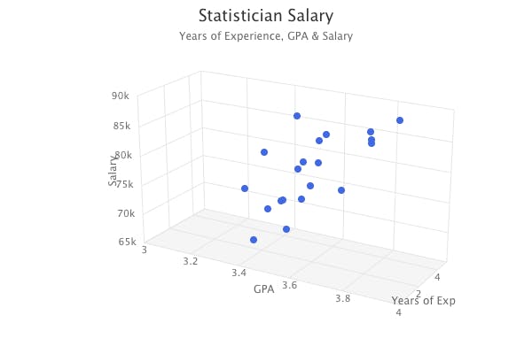
For example, let’s take the statistician salary dataset, add a new predictor for college GPA, and add 10 new data points.

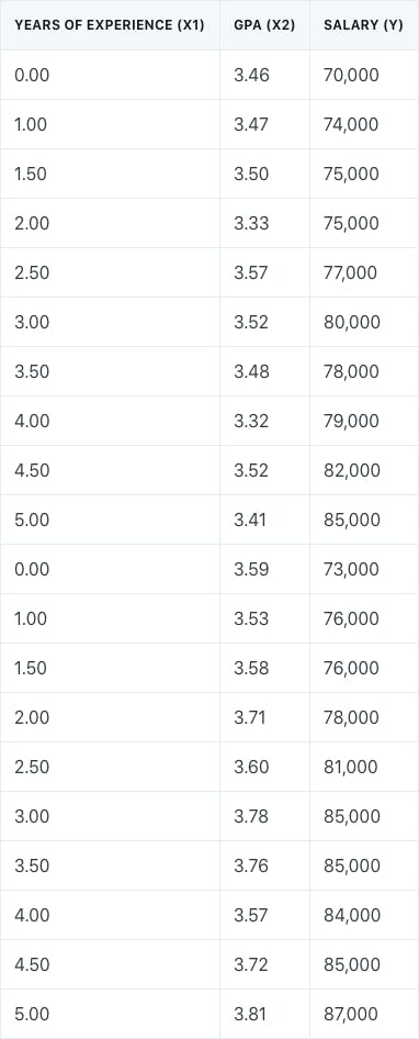
The multiple linear regression model for the dataset would take the form:

The multiple linear regression model would fit a plane to the dataset. The dataset is represented below as a 3D scatter plot with an X, Y, and Z axis.

In multiple linear regression, we’re interested in a few specific questions:

1. Is at least one of the predictors useful in predicting the response?
2. Do all of the predictors help explain Y, or only a few of them?
3. How well does the model fit the data?
4. How accurate is our prediction?

Least Squares Criteria

Similar to simple linear regression, the coefficient estimates in multiple linear regression are chosen based on the same least squares approach that minimizes RSS.

Interpretation of β Coefficients​

The interpretation of the coefficients is also very similar to the simple linear regression setting, with one key difference (indicated in bold). In general, we say that:

• If all of the predictors were 0, the prediction (Y) would be β₀, on average.
• For every one increase in some predictor Xⱼ, the prediction changes by βⱼ, on average, holding all of the other predictors constant.

Hypothesis Testing

So, how do we determine whether or not there truly is a relationship between the _X_s and Y? In other words, how do we know that the _X_s are actually good predictors for Y?

Similar to the simple linear regression setting, we perform a hypothesis test. The null and alternative hypotheses are slightly different:

• Null Hypothesis: No relationship between the _X_s and Y
• Alternative Hypothesis: At least one predictor has a relationship to the response

F-statistic and p-value

So, how do we determine if at least one βⱼ is non-zero? In simple regression, we determined the t-statistic. In multiple regression, we determine the F-statistic instead.

When there is no relationship between the response and predictors, we generally expect the F-statistic to be close to 1.

If there is a relationship, we generally expect the F-statistic to be greater than 1.

Similar to the t-statistic, the F-statistic also allows us to determine the p-value, which ultimately helps decide whether or not a relationship exists.

The p-value is essentially interpreted in the same way that it is interpreted in simple regression.

Typically, we want p-values less than 5% or 1% to reject the null hypothesis. In other words, rejecting the null hypothesis means that we are declaring that some relationship exists between the _X_s and Y.

t-statistics in Multiple Linear Regression

In multiple linear regression, we will receive outputs that indicate the t-statistic and p-values for each of the different coefficients.

However, we have to use the overall F-statistic instead of the individual coefficient p-values. This is because when the number of predictors is large (e.g. p=100), about 5% of the coefficients will have low p-values less than 5% just by chance. Therefore, in this scenario, choosing whether or not to reject the null hypothesis based on the individual p-values would be flawed.

Determining Variable Significance

So, after concluding that at least one predictor is related to the response, how do we determine which specific predictors are significant?

This process is called variable selection, and there are three approaches: forward selection, backward selection, and mixed selection.

Forward Selection

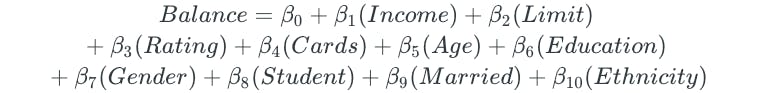
Assume that we had a dataset of credit card balance and 10 predictors.

Forward selection begins with a null model with no predictors:

Then, 10 different simple linear regression models are built for each of the predictors:

The predictor that results in the lowest RSS is then added to the initial null model. Assume that the Limit variable is the variable that results in the lowest RSS. The forward selection model would then become:

Then, a second predictor is added to this new model, which will result in building 9 different multiple linear regression models for the remaining predictors:

The second predictor that results in the lowest RSS is then added to the model. Assume that the model with the Income variable resulted in the lowest RSS. The forward selection model would then become:

This process of adding predictors is continued until some statistical stopping rule is satisfied.

Backward Selection

Backward selection begins with a model with all predictors:

Then, the variable with the largest p-value is removed, and the new model is fit.

Again, the variable with the largest p-value is removed, and the new model is fit.

This process is continued until some statistical stopping rule is satisfied, such as all variables in the model having low p-values less than 5%.

Mixed Selection

Mixed selection is a combination of forward and backward selection. We begin with a null model that contains no predictors. Then, variables are added one by one, exactly as done in forward selection. However, if at any point the p-value for some variable rises above a chosen threshold, then it is removed from the model, as done in backward selection.

Assessing Model Accuracy

Similar to the simple regression setting, RSE and R² are used to determine how well the model fits the data.

RSE

In multiple linear regression, RSE is calculated as follows:

R-Squared (R²)

R² is interpreted in the same manner that it is interpreted in simple regression.

However, in multiple linear regression, adding more predictors to the model will always result in an increase in R².

Therefore, it is important to look at the magnitude at which R² changes when adding or removing a variable. A small change will generally indicate an insignificant variable, whereas a large change will generally indicate a significant variable.

Assessing Prediction Accuracy

How do we estimate how accurate the actual predictions are? Confidence intervals and prediction intervals can help assess prediction accuracy.

Confidence Intervals

Confidence intervals are determined through the β coefficient estimates and their inaccuracy through the standard errors.

This means that confidence intervals only account for reducible error.

Prediction Intervals

Reducible error isn’t the only type of error that is present in regression modeling.

Even if we knew the true values of the β coefficients, we would not be able to predict the response variable perfectly because of random error ϵ in the model, which is an irreducible error.

Prediction intervals go a step further than confidence intervals by accounting for both reducible and irreducible error. This means that prediction intervals will always be wider than confidence intervals.

Other Considerations in Regression Modeling

Qualitative Predictors

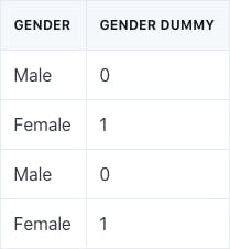
It is possible to have qualitative predictors in regression models. For example, assume that we had a predictor that indicated gender.

For qualitative variables with only two levels, we could simply create a “dummy” variable that takes on two values:

We’d simply use that logic to create a new column for the dummy variable in the data, and use that for regression purposes:

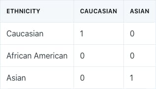
But what if the qualitative variable had more than two levels? For example, assume we had a predictor that indicated ethnicity:

In this case, a single dummy variable cannot represent all of the possible values. In this situation, we create multiple dummy variables:

For qualitative variables with multiple levels, there will always be one fewer dummy variable than the total number of levels. In this example, we have three ethnicity levels, so we create two dummy variables.

The new variables for regression purposes would be represented as follows:

Extensions of the Linear Model

Regression models provide interpretable results and work well, but make highly restrictive assumptions that are often violated in practice.

Two of the most important assumptions state that the relationship between the predictors and response are additive and linear.

The additive assumption means that the effect of changes in some predictor Xⱼ on the response is independent of the values of the other predictors.

The linear assumption states that the change in the response Y due to a one-unit change in some predictor Xⱼ is constant, regardless of the value of Xⱼ.

Removing the Additive Assumption

Assume that we had an advertising dataset of money spent on TV ads, money spent on radio ads, and product sales.

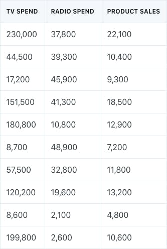
The multiple linear regression model for the data would have the form:

This model states that the average effect on sales for a $1 increase in TV advertising spend is β₁, on average, regardless of the amount of money spent on radio ads.

However, it is possible that spending money on radio ads actually increases the effectiveness of TV ads, thus increasing sales further. This is known as an interaction effect or a synergy effect. The interaction effect can be taken into account by including an interaction term:

The interaction term relaxes the additive assumption. Now, every $1 increase in TV ad spend increases sales by β₁ + β₃(Radio).

Sometimes it is possible for the interaction term to have a low p-value, yet the main terms no longer have a low p-value. The hierarchical principle states that if an interaction term is included, then the main terms should also be included, even if the p-values for the main terms are not significant.

Interaction terms are also possible for qualitative variables, as well as a combination of qualitative and quantitative variables.

Non-Linear Relationships

In some cases, the true relationship between the predictors and response may be non-linear. A simple way to extend the linear model is through polynomial regression.

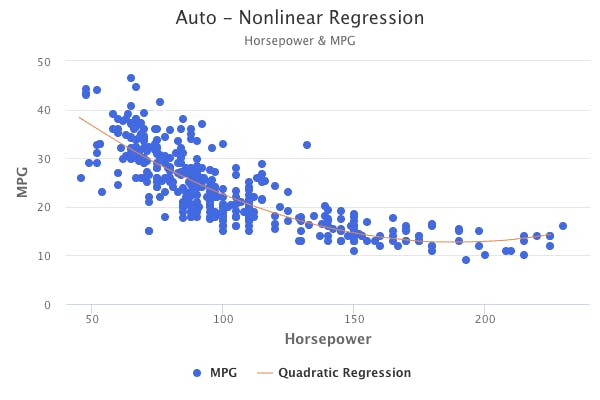
For example, for automobiles, there is a curved relationship between miles per gallon and horsepower.

A quadratic model of the following form would be a great fit to the data:

Potential Problems with Linear Regression

When fitting linear models, there are six potential problems that may occur: non-linearity of data, correlation of error terms, nonconstant variance of error terms, outliers, high leverage data points, and collinearity.

Non-Linearity of Data

Residual plots are a useful graphical tool for the identification of non-linearity.

In simple linear regression, the residuals are plotted against the predictor.

In multiple linear regression, the residuals are plotted against the predicted values.

If there is some kind of pattern in the residual plot, then it is an indication of potential non-linearity.

Non-linear transformations, such as log-transformation, of the predictors could be a simple method to solving the issue.

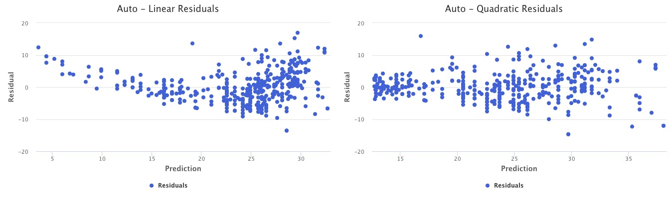
For example, take a look at the below residual graphs, which represent different types of fits for the automobile data mentioned previously. The graph on the left represents what the residuals look like if a simple linear model is fit to the data. Clearly, there is a curved pattern in the residual plot, indicating non-linearity. The graph on the right represents what the residuals look like if a quadratic model is fit to the data. Fitting a quadratic model seems to resolve the issue, as a pattern doesn’t exist in the plot.

Correlation of Error Terms

Proper linear models should have residual terms that are uncorrelated. This means that the sign (positive or negative) of some residual should provide no information about the sign of the next residual.

If the error terms are correlated, we may have an unwarranted sense of confidence in the linear model.

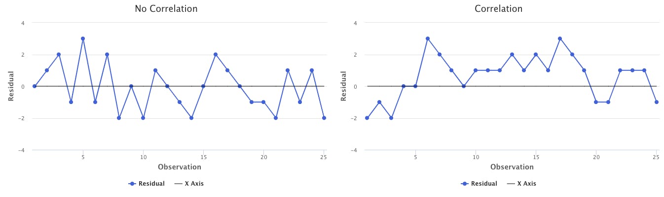
To determine if correlated errors exist, we plot residuals in order of observation number. If the errors are uncorrelated, there should not be a pattern. If the errors are correlated, then we may see tracking in the graph. Tracking is where adjacent residuals have similar signs.

For example, take a look at the below graphs. The graph on the left represents a scenario in which residuals are not correlated. In other words, just because one residual is positive doesn’t seem to indicate that the next residual will be positive. The graph on the right represents a scenario in which the residuals are correlated. There are 15 residuals in a row that are all positive.

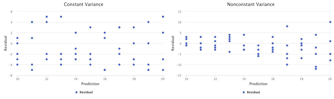
Nonconstant Variance of Error Terms

Proper linear models should also have residual terms that have a constant variance. The standard errors, confidence intervals, and hypothesis tests associated with the model rely on this assumption.

Nonconstant variance in errors is known as heteroscedasticity. It is identified as the presence of a funnel shape in the residual plot.

One solution to nonconstant variance is to transform the response using a concave function, such as log(Y) or the square root of Y. Another solution is to use weighted least squares instead of ordinary least squares.

The graphs below represent the difference between constant and nonconstant variance. The residual plot on the right has a funnel shape, indicating nonconstant variance.

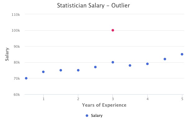
Outliers

Depending on how many outliers are present and their magnitude, they could either have a minor or major impact on the fit of the linear model. However, even if the impact is small, they could cause other issues, such as impacting the confidence intervals, p-values, and R².

Outliers are identified through various methods. The most common is studentized residuals, where each residual is divided by its estimated standard error. Studentized residuals greater than 3 in absolute value are possible outliers.

These outliers can be removed from the data to come up with a better linear model. However, it is also possible that outliers indicate some kind of model deficiency, so caution should be taken before removing the outliers.

The red data point below represents an example of an outlier that would greatly impact the slope of a linear regression model.

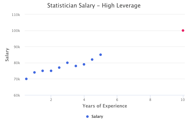
High Leverage Data Points

Observations with high leverage have an unusual value compared to the other observation values. For example, you might have a dataset of X values between 0 and 10, and just one other data point with a value of 20. The value of 20 is a high leverage data point.

High leverage is determined through the leverage statistic. The leverage statistic is always between 1/n and 1.

The average leverage is defined as:

If the leverage statistic of a data point is greatly higher than the average leverage, then we have reason to suspect high leverage.

The red data point below represents an example of a high leverage data point that would impact the linear regression fit.

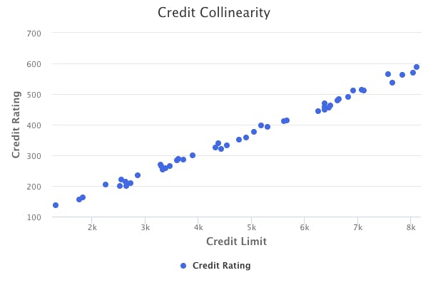
Collinearity

Collinearity refers to the situation in which 2 or more predictor variables are closely related. Collinearity makes it difficult to separate out the individual effects of collinear variables on the response. It also reduces the accuracy of the estimates of the regression coefficients by causing the coefficient standard errors to grow, thus reducing the credibility of hypothesis testing.

A simple way to detect collinearity is to look at the correlation matrix of the predictors.

However, not all collinearity can be detected through the correlation matrix. It is possible for collinearity to exist between multiple variables instead of pairs of variables, which is known as multicollinearity.

The better way to assess collinearity is through the Variance Inflation Factor (VIF). VIF is the ratio of the variance of a coefficient when fitting the full model, divided by the variance of the coefficient when fitting a model only on its own. The smallest possible VIF is 1. In general, a VIF that exceeds 5 or 10 may indicate a collinearity problem.

One way to solve the issue of collinearity is to simply drop one of the predictors from the linear model. Another solution is to combine collinear variables into one variable.

The chart below demonstrates an example of collinearity. As we know, an individual’s credit limit is directly related to their credit rating. A dataset that includes both of these predictor should only include one of them for regression purposes, to avoid the issue of collinearity.

Originally published at https://www.bijenpatel.com on August 3, 2020.

I will be releasing the equivalent Python code for these examples soon. Subscribe to get notified!

ISLR Chapter 3 — R Code

Simple Linear Regression

library(MASS) # For model functions
library(ISLR) # For datasets
library(ggplot2) # For plotting

# Working with the Boston dataset to predict median house values
head(Boston)

# Fit a simple linear regression model
# Median house value is the response (Y)
# Percentage of low income households in the neighborhood is the predictor
Boston_lm = lm(medv ~ lstat, data=Boston)

# View the fitted simple linear regression model
summary(Boston_lm)

# View all of the objects stored in the model, and get one of them, such as the coefficients
names(Boston_lm)
Boston_lm$coefficients

# 95% confidence interval of the coefficients
confint(Boston_lm, level=0.95)

# Use the model to predict house values for specific lstat values
lstat_predict = c(5, 10, 15)
lstat_predict = data.frame(lstat=lstat_predict)

predict(Boston_lm, lstat_predict) # Predictions
predict(Boston_lm, lstat_predict, interval="confidence", level=0.95)
predict(Boston_lm, lstat_predict, interval="prediction", level=0.95)

# Use ggplot to create a residual plot of the model
Boston_lm_pred_resid = data.frame(Prediction=Boston_lm$fitted.values, Residual=Boston_lm$residuals)

Boston_resid_plot = ggplot(Boston_lm_pred_resid, aes(x=Prediction, y=Residual)) +
  geom_point() +
  labs(title="Boston Residual Plot", x="House Value Prediction", y="Residual")

plot(Boston_resid_plot)

# Use ggplot to create a studentized residual plot of the model (for outlier detection)
Boston_lm_pred_Rstudent = data.frame(Prediction=Boston_lm$fitted.values, Rstudent=rstudent(Boston_lm))

Boston_Rstudent_plot = ggplot(Boston_lm_pred_Rstudent, aes(x=Prediction, y=Rstudent)) +
  geom_point() +
  labs(title="Boston Rstudent Plot", x="House Value Prediction", y="Rstudent")

plot(Boston_Rstudent_plot)

# Determine leverage statistics for the lstat values (for high leverage detection)
Boston_leverage = hatvalues(Boston_lm)
head(order(-Boston_leverage), 10)</span>

Multiple Linear Regression

# Multiple linear regression model with two predictors
# Median house value is the response (Y)
# Percentage of low income households in the neighborhood is the first predictor (X1)
# Percentage of houses in the neighborhood built before 1940 is the second predictor (X2)
Boston_lm_mult_1 = lm(medv ~ lstat + age, data=Boston)
summary(Boston_lm_mult_1)
## Coefficients:
## (Intercept)        lstat          age  
##    33.22276     -1.03207      0.03454

# Multiple linear regression model with all predictors
# Median house value is the response (Y)
# Every variable in the Boston dataset is a predictor (X)
Boston_lm_mult_2 = lm(medv ~ ., data=Boston)

# Multiple linear regression model with all predictors except specified (age)
Boston_lm_mult_3 = lm(medv ~ . -age, data=Boston)

# Multiple linear regression model with an interaction term
Boston_lm_mult_4 = lm(medv ~ crim + lstat:age, data=Boston)
# The colon ":" will include an (lstat)(age) interaction term

Boston_lm_mult_5 = lm(medv ~ crim + lstat*age, data=Boston)
# The asterisk "*" will include an (lstat)(age) interaction term
# It will also include the terms by themselves, without having to specify separately

# Multiple linear regression model with nonlinear transformation
Boston_lm_mult_6 = lm(medv ~ lstat + I(lstat^2), data=Boston)

# Multiple linear regression model with nonlinear transformation (easier method)
Boston_lm_mult_7 = lm(medv ~ poly(lstat, 5), data=Boston)

# Multiple linear regression model with log transformation
Boston_lm_mult_8 = lm(medv ~ log(rm), data=Boston)

# ANOVA test to compare two different regression models
anova(Boston_lm_mult, Boston_lm_mult_6)
# Null Hypothesis: Both models fit the data equally well
# Alternative Hypothesis: The second model is superior to the first

# 95% confidence interval for the coefficients
confint(Boston_lm_mult_1, level=0.95)</span>

Linear Regression with Qualitative Variables

# The Carseats data has a qualitative variable for the quality of shelf location
# It takes on one of three values: Bad, Medium, Good
# R automatically generates dummy variables ShelveLocGood and ShelveLocMedium

# Multiple linear regression model to predict carseat sales
Carseats_lm_mult = lm(Sales ~ ., data=Carseats)
summary(Carseats_lm_mult)
## Coefficients:
##                   Estimate Std. Error t value Pr(>|t|)    
## ...
## ShelveLocGood    4.8501827  0.1531100  31.678  < 2e-16 ***
## ShelveLocMedium  1.9567148  0.1261056  15.516  < 2e-16 ***
## ...</span>