This is a summary of chapter 8 of the Introduction to Statistical Learning textbook. I’ve written a 10-part guide that covers the entire book. The guide can be read at my website, or here at Hashnode. Subscribe to stay up to date on my latest Data Science & Engineering guides!

Tree-based methods for regression and classification involve segmenting the predictor space into a number of simple regions. To make a prediction for an observation, we simply use the mean or mode of the training observations in the region that it belongs to. Since the set of splitting rules used to segment the predictor space can be summarized in a tree, these approaches are known as decision tree methods.

These methods are simple and useful for interpretation, but not competitive in terms of prediction accuracy when compared with the methods from the chapter on linear model selection and regularization. However, advanced methods such as bagging, random forests, and boosting can result in dramatic improvements at the expense of a loss in interpretation.

Basics of Decision Trees

Regression Trees

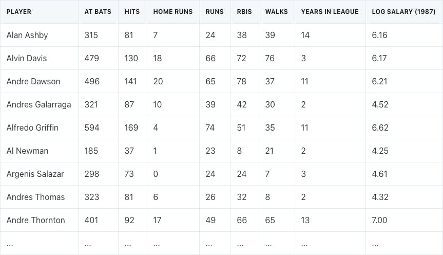
Assume that we had a baseball salary dataset that consisted of the number of years that a player was in the league, the number of hits in the previous year, and each player’s log-transformed salary.

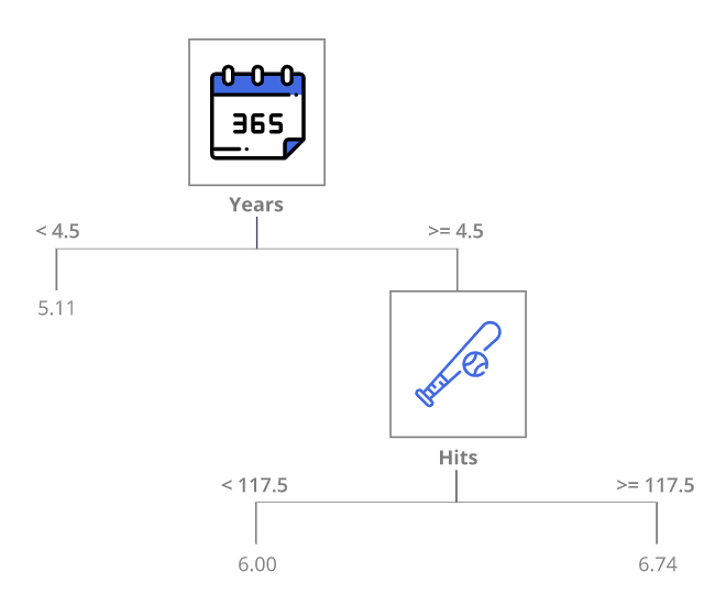
We might get a decision tree that looks like the following:

The interpretation of the tree might look as follows:

• Years is the most important factor in determining salary — players with less experience earn less money
• If a player is experienced (more than 5 years in the league), then the number of hits plays a role in the salary

The tree is probably an oversimplification of the relationship, but is easy to interpret and has a nice graphical representation.

In general, the process of building a regression tree is a two-step procedure:

1. Divide the predictor space (the set of possible values for all Xⱼ into j distinct and non-overlapping regions (R₁, R₂, R₃ … Rⱼ)
2. For every observation that falls into some region, we make the same prediction, which is the mean of the response values in the region

The regions are constructed by dividing the predictor space into “box” shapes for simplicity and ease of interpretation. The goal is to find boxes that minimize the RSS given by the following:

Unfortunately, it is computationally infeasible to consider every partition of the feature space. Therefore, we take a greedy top-down approach known as recursive binary splitting. First, we consider all of the predictors and all of the possible cutpoints (s) for each of the predictors and choose the predictor and cutpoint that results in the lowest RSS. Next, the process is repeated to further split the data, but this time we split one of the two previously identified regions, which results in 3 total regions. The process continues until some stopping criteria is reached.

However, the process may end up overfitting the data and result in a tree that is too complex. A smaller tree would result in lower variance and easier interpretation at the cost of a little more bias. Therefore, we should first grow a large complex tree, and then prune it back to obtain a subtree.

This is done through a method known as cost complexity pruning, or weakest link pruning. The method allows us to consider a small set of subtrees instead of every possible subtree. This is done through the addition of a tuning parameter, α. For each value of α, there is a subtree T such that the following is as small as possible:

• Where |T| is the number of terminal nodes
• Where R is the rectangle corresponding to the m-th terminal node

The α tuning parameter controls a tradeoff between tree complexity and its fit to the data. As α increases, there is a price to pay for having a tree with many terminal nodes, so the equation will typically be minimized for a smaller subtree. This is similar to the lasso regression method, which controlled the complexity of the linear model. As α is increased from zero, the branches get pruned in a nested and predictable fashion, so getting the subtree as a function of α is simple. The final value of α is selected using cross-validation.

Classification Trees

Classification trees are similar to regression trees, but predict qualitative responses. In regression, the prediction for some observation is given by the mean response of the observations at some terminal node. In classification, the prediction is given by the most commonly occurring class at the terminal node.

In classification, instead of using the RSS, we look at either the Gini index or the cross-entropy. Both are very similar measures, where small values indicate node purity, meaning that a node contains predominantly observations from a single class. Either of these measures can be used to build a tree and evaluate splits.

When it comes to pruning a tree, we could either use the Gini index, cross-entropy, or the classification error rate. The classification error rate is the fraction of observations in a region that do not belong to the most common class. The classification error rate may be preferable for the purposes of prediction accuracy and tree pruning.

Qualitative Variables

In a dataset, we may have a qualitative variable that takes on more than two values, such as an ethnicity variable.

In a decision tree, these variables are typically split through the use of letters or numbers that are assigned to the values of the qualitative variable.

Pros & Cons of Trees

The advantage of decision trees over other methods is their simplicity. Decision trees are very easy to explain to others, and closely mirror human decision-making. They can be displayed graphically and easily interpreted by non-experts.

The disadvantage is that the ease of interpretation comes at the cost of prediction accuracy. Usually, other regression and classification methods are more accurate.

However, advanced methods such as bagging, random forests, and boosting can greatly improve predictive performance at the cost of interpretability.

Bagging, Random Forests, and Boosting

Bagging

Bagging is a general purpose method for reducing the variance of a statistical learning method. It is very useful for decision trees because they suffer from high variance.

A natural way to reduce variance and increase prediction accuracy is to take many training sets from the population, build separate trees using each dataset, and average the predictions. However, it isn’t practical to do this because we usually never have access to multiple different training datasets. Instead, we can use the bootstrap method to generate B different bootstrapped training datasets, create B trees, and average the predictions. In classification, instead of averaging the predictions, we take a majority vote, where the overall prediction is the most occurring class.

In bagging, the trees are grown large and are not pruned. Additionally, there is a straightforward way to estimate the test error of a bagged model without needing to perform cross-validation. Remember that bootstrapped datasets are created through resampling, which allows for observations to be repeated. As it turns out, on average, each bagged tree will make use of two-thirds of the total observations because of the resampling. The remaining one-third of the observations not used to fit a tree are referred to as the out-of-bag (OOB) observations. We predict the response for the i-th observation using each tree in which the i-th observation was OOB and average the predictions or take a majority vote. This is done for all of the observations in the original dataset, and the overall test error rate is then determined.

Bagging improves prediction accuracy at the expense of interpretability. However, we can obtain an overall summary of the importance of each predictor using RSS or the Gini index. This is done by recording the total amount that the RSS or Gini index decreases due to splits in a given predictor and averaging over all of the trees. The larger the total value, the more significant the predictor.

Random Forests

Random forests provide an improvement over bagging by decorrelating the trees. The random forest method is similar to bagging, where a large number of trees are built on bootstrapped datasets. However, when building the trees, each time a split is considered, a random sample of m predictors is chosen as split candidates from the full set of p predictors, and the split can only use one of the m predictors. Additionally, a fresh set of m predictors is taken at each split. Usually, we use m = sqrt(p).

Why might only considering a subset of the predictors at each split be a good thing? Suppose that we have a dataset with one very strong predictor and some other moderately strong predictors. In the bagged trees, almost every tree will use the very strong predictor as the top split. All of the bagged trees will look very similar and be highly correlated. Averaging many highly correlated trees does not result in a large reduction to variance. Since random forests force each split to consider only a subset of the predictors, many splits will not even consider the strongest predictor. Basically, this decorrelates the trees and reduces variance.

Boosting

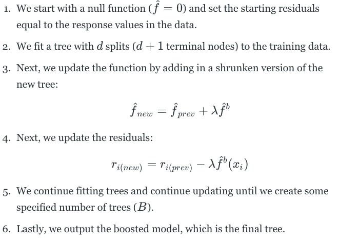
Like bagging, boosting is a general approach that can be applied to many different statistical learning methods. Boosting involves building many trees, but each tree is grown sequentially. This means that each tree is grown using information from a previously grown tree. Additionally, boosting does not involve bootstrap sampling. Each tree is fit on a modified version of the original dataset. Boosting works as follows:

The boosting approach learns slowly. If we set the parameter d to be small, we fit small trees to the residuals and slowly improve the function in areas where it does not perform well. The shrinkage parameter λ slows the process down even further, allowing more and different shaped trees to attack the residuals.

In boosting, unlike in bagging, the construction of each tree depends strongly on the trees already grown. Additionally, boosting could potentially overfit the data if the number of trees B is too large. Therefore, we use cross-validation to select B. Typically, λ is between 0.01 and 0.001, and d=1 is usually sufficient.

Originally published at https://www.bijenpatel.com on August 8, 2020.

I will be releasing the equivalent Python code for these examples soon. Subscribe to get notified!

ISLR Chapter 8 — R Code

Classification Trees

library(ISLR)
library(MASS)
library(ggplot2)
library(gridExtra) # For side-by-side ggplots
library(e1071)
library(caret)

library(tree) # For decision trees

# We will work with the Carseats data
# It contains data on sales of carseats for 400 different store locations
head(Carseats)

# We will build a tree that predicts whether or not a location had "high" sales
# We define "high" as sales exceeding 8000 units

# Create a vector to indicate whether or not a location had "high" sales
High = ifelse(Carseats$Sales <= 8, "No", "Yes")

# Merge the vector to the entire Carseats data
Carseats = data.frame(Carseats, High)

# The tree function is used to fit a decision tree
Carseats_tree = tree(High ~ . -Sales, data=Carseats)

# Use the summary function to see the predictors used, # of terminal nodes, and training error
summary(Carseats_tree)

# Visualize the tree model
plot(Carseats_tree)
text(Carseats_tree, pretty=0) # pretty=0 shows category names instead of letters

# To estimate test error, we fit a tree to training data and predict on test data
set.seed(2)

train = sample(1:400, 200)
Carseats_train = Carseats[train,]
Carseats_test = Carseats[-train,]

Carseats_tree = tree(High ~ . -Sales, data=Carseats_train)
Carseats_tree_predictions = predict(Carseats_tree, Carseats_test, type="class")

# Use a confusion matrix to determine the accuracy of the tree model
confusionMatrix(Carseats_tree_predictions, Carseats_test$High, positive="Yes")</span>

Tree Pruning

# Will pruning the tree lead to improved accuracy?
# The cv.tree function performs cross-validation to determine the optimal tree complexity
set.seed(3)
Carseats_tree_cv = cv.tree(Carseats_tree, FUN=prune.misclass)
    # FUN = prune.misclass performs pruning through the misclassification error rate

# The object contains different terminal node values, their error rate, and cost complexity parameter
Carseats_tree_cv

# Create a dataframe of the values from the cv.tree function
Carseats_tree_cv_df = data.frame(Nodes=Carseats_tree_cv$size,
                                Error=Carseats_tree_cv$dev,
                                Alpha=Carseats_tree_cv$k)

# Plot the number of terminal nodes, and their corresponding errors and alpha parameters
Carseats_tree_cv_error = ggplot(Carseats_tree_cv_df, aes(x=Nodes, y=Error)) + geom_line() + geom_point()
Carseats_tree_cv_alpha = ggplot(Carseats_tree_cv_df, aes(x=Nodes, y=Alpha)) + geom_line() + geom_point()

# Show the plots side-by-side with the grid.arrange function from gridExtra package
grid.arrange(Carseats_tree_cv_error, Carseats_tree_cv_alpha, ncol=2)
    # A tree with 9 terminal nodes results in the lowest error
    # This also corresponds to alpha value of 1.75

# Finally, prune the tree with prune.misclass function and specify 9 terminal nodes
Carseats_tree_pruned = prune.misclass(Carseats_tree, best=9)

# Plot the pruned tree
plot(Carseats_tree_pruned)
text(Carseats_tree_pruned, pretty=0)

# Use the pruned tree to make predictions, and compare the accuracy to the non-pruned tree
Carseats_tree_pruned_predictions = predict(Carseats_tree_pruned, Carseats_test, type="class")
confusionMatrix(Carseats_tree_pruned_predictions, Carseats_test$High, positive="Yes")
  # 77% accuracy for the pruned tree versus 71.5% for the non-pruned tree
  # Pruning results in a better model</span>

Regression Trees

# We will work with the Boston data, which has data on median house values
head(Boston)

# We will build a tree that predicts median house values

# First, create training and test datasets
set.seed(1)

train = sample(1:nrow(Boston), nrow(Boston)/2)
Boston_train = Boston[train,]
Boston_test = Boston[-train,]

# Fit a tree to the training data
Boston_tree = tree(medv ~ ., Boston_train)

# See the predictors used, number of terminal nodes, and error
summary(Boston_tree)

# Plot the tree
plot(Boston_tree)
text(Boston_tree, pretty=0)

# Perform cross validation to determine optimal tree complexity
Boston_tree_cv = cv.tree(Boston_tree)

# Create a dataframe of the values from cross-validation
Boston_tree_cv_df = data.frame(Nodes=Boston_tree_cv$size, Error=Boston_tree_cv$dev, Alpha=Boston_tree_cv$k)

# Plot the number of terminal nodes, and their corresponding errors and alpha parameters
Boston_tree_cv_error = ggplot(Boston_tree_cv_df, aes(x=Nodes, y=Error)) + geom_line() + geom_point()
Boston_tree_cv_alpha = ggplot(Boston_tree_cv_df, aes(x=Nodes, y=Alpha)) + geom_line() + geom_point()

grid.arrange(Boston_tree_cv_error, Boston_tree_cv_alpha, ncol=2)

# Cross-validation indicates that a tree with 8 terminal nodes is best
# However, we could choose to use 7, as the error for 7 is essentially nearly the same as 8
# This will result in a simpler tree
Boston_pruned_tree = prune.tree(Boston_tree, best=7)

# Plot the final pruned tree
plot(Boston_pruned_tree)
text(Boston_pruned_tree, pretty=0)

# Use the pruned tree to make predictions on the test data, and determine the test MSE
Boston_tree_predictions = predict(Boston_pruned_tree, Boston_test)
mean((Boston_tree_predictions - Boston_test$medv)^2)</span>

Bagging

library(randomForest) # The randomForest package is used for bagging and random forest

# We continue working with the Boston data

# The randomForest function is used to perform both bagging and random forest
# Bagging is a special case of random forest, where all predictors are used
set.seed(1)
Boston_bag = randomForest(medv ~ ., data=Boston_train, mtry=13, importance=TRUE)

# Use the bagged tree to make predictions on the test data
Boston_bag_predictions = predict(Boston_bag, Boston_test)

# Determine the test MSE
mean((Boston_bag_predictions - Boston_test$medv)^2)</span>

Random Forest

# We continue working with the Boston data

# For random forest, we simply specify a smaller number of predictors in mtry
# Typically, m=(p/3) is used for regression
# Typically, m=sqrt(p) is used for classification
set.seed(1)
Boston_rf = randomForest(medv ~ ., data=Boston_train, mtry=round(13/3), importance=TRUE)

# Use the bagged tree to make predictions on the test data
Boston_rf_predictions = predict(Boston_rf, Boston_test)

# Determine the test MSE and compare to the result from bagging
mean((Boston_rf_predictions - Boston_test$medv)^2)
  # Lower test MSE than result from bagging

# The importance function can be used to see the importance of each variable
# The first column indicates how much the error increases if the variable is excluded from the model
# The second column indicates how much node purity decreases if the variable is excluded from the model
importance(Boston_rf)

# Quick plot of the data from the importance function
varImpPlot(Boston_rf)
  # lstat and rm are the most importance variables</span>

Boosting

library(gbm) # For boosting

# We continue working with the Boston data

# The gbm function is used to perform boosting
# For regression problems, the distribution is set to gaussian
# For classification problems, the distribution is set to bernoulli
# n.trees is used to specify the number of trees
# interaction.depth is used to limit the depth of each tree
set.seed(1)
Boston_boost = gbm(medv ~ ., Boston_train, distribution="gaussian", n.trees=5000, interaction.depth=4)

# The summary function shows the relative influence statistics for each variable
summary(Boston_boost)

# Plot the marginal effect of variables on the response after integrating out the other variables
plot(Boston_boost, i="lstat")
plot(Boston_boost, i="rm")

# Use the boosted model to predict on the test data
Boston_boost_predictions = predict(Boston_boost, Boston_test, n.trees=5000, interaction.depth=4)

# Determine the test MSE
mean((Boston_boost_predictions - Boston_test$medv)^2)
  # Boosting results in a test MSE that is slightly better than random forest</span>