This is a summary of chapter 4 of the Introduction to Statistical Learning textbook. I’ve written a 10-part guide that covers the entire book. The guide can be read at my website, or here at Hashnode. Subscribe to stay up to date on my latest Data Science & Engineering guides!

Overview of Classification

Qualitative variables, such as gender, are known as categorical variables. Predicting qualitative responses is known as classification.

Some real world examples of classification include determining whether or not a banking transaction is fraudulent, or determining whether or not an individual will default on credit card debt.

The three most widely used classifiers, which are covered in this post, are:

• Logistic Regression
• Linear Discriminant Analysis
• K-Nearest Neighbors

There are also more advanced classifiers, which are covered later:

• Generalized Additive Models
• Trees
• Random Forests
• Boosting
• Support Vector Machines

Logistic Regression

Logistic regression models the probability that the response Y belongs to a particular category.

For example, assume that we have data on whether or not someone defaulted on their credit. The data includes one predictor for the credit balance that someone had.

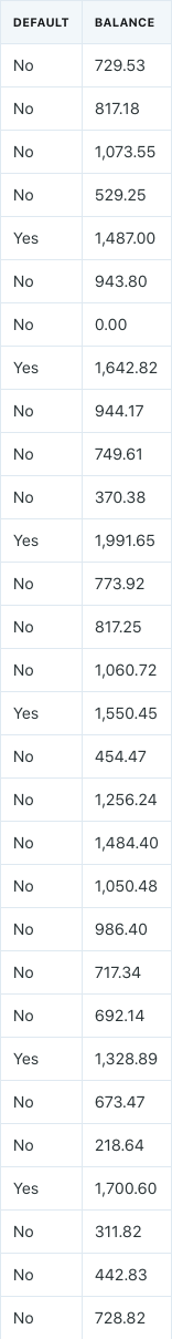
Logistic regression would model the probability of default, given credit balance:

Additionally, a probability threshold can be chosen for the classification.

For example, if we choose a probability threshold of 50%, then we would indicate any observation with a probability of 50% or more as “default.”

However, we could also choose a more conservative probability threshold, such as 10%. In this case, any observation with a probability of 10% or more would be indicated as “default.”

Logistic Model

The logistic function is used to model the relationship between the probability (Y) and some predictor (X) because the function falls between 0 and 1 for all X values. The logistic function has the form:

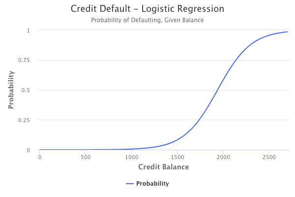
The logistic function always produces an S-shaped curve.

Additionally, the logistic function can also be rewritten as a logit function:

The logistic regression model for Credit Default data may look like the chart below.

Interpretation of Coefficients

This equation can be interpreted as a one unit increase in X changing the log-odds or logit (left side of equation) by β₁.

The fraction inside the log() is known as the odds. In the context of the Credit Default data, the odds would indicate the ratio of the probability of defaulting versus the probability of not defaulting. For example, on average, 1 in 5 people with an odds of 1/4 will default. On the other hand, on average, 9 out of 10 people with an odds of 9/1 will default.

So, alternatively, the logit function can also be interpreted as a one-unit increase in X multiplying the odds by e^β₁.

β₁ cannot be interpreted as a specific change in value for the probability. The only conclusion that can be made is that if the coefficient is positive, then an increase in X will increase the probability, whereas if the coefficient is negative, then an increase in X will decrease the probability.

Maximum Likelihood

The coefficients are estimated through the maximum likelihood method.

In the context of the Credit Default data, the maximum likelihood estimate essentially attempts to find β₀ and β₁ such that plugging these estimates into the logistic function results in a number close to 1 for individuals who defaulted, and a number close to 0 for individuals who did not default.

In other words, maximum likelihood chooses coefficients such that the predicted probability of each observation in the data corresponds as closely as possible to the actual observed status.

Hypothesis Testing

So, how do we determine whether or not there truly is a relationship between the probability of a class and some predictor?

Similar to the linear regression setting, we conduct a hypothesis test:

z-statistic and p-value

In logistic regression, we have a z-statistic instead of the t-statistic that we had in linear regression. However, they are essentially the same.

The z-statistic measures the number of standard deviations that β₁ is away from 0.

The z-statistic allows us to determine the p-value, which ultimately helps determine whether or not the coefficient is non-zero.

The p-value indicates how likely it is to observe a meaningful association between the probability of a class and some predictor X by some bizarre random error or chance, as opposed to there being a true relationship between them.

Typically, we want p-values less than 5% or 1% to reject the null hypothesis. In other words, rejecting the null hypothesis means that we are declaring that some relationship exists.

Multiple Logistic Regression

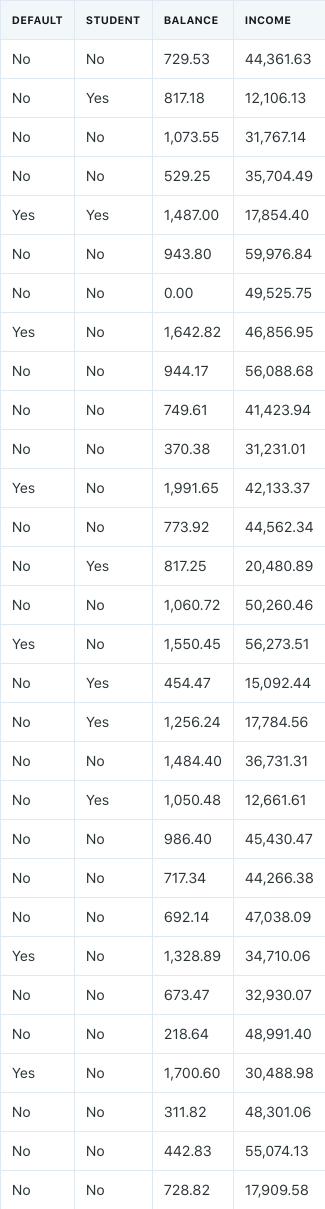
What if our dataset had multiple predictors. For example, let’s expand our Credit Default dataset to include two additional predictors: student status and income.

Logistic Model

Similar to how the simple linear regression model was extended to multiple linear regression, the logistic regression model is extended in a related fashion:

Interpretation of Coefficients

The interpretation of the coefficients remains nearly the same. However, when interpreting one of the coefficients, we have to indicate that the values of the other predictors remain fixed.

Logistic Regression for Multiple Response Classes

What if we had to classify observations in more than two classes? In the Credit Default data, we only had two classes: Default and No Default.

For example, assume that we had a medical dataset and had to classify medical conditions as either a stroke, drug overdose, or seizure.

The two-class logistic regression models have multiple-class extensions, but are not used often.

Discriminant analysis is the popular approach for multiple-class classification.

Linear Discriminant Analysis

Linear discriminant analysis is an alternative approach to classification that models the distributions of the different predictors separately in each of the response classes (Y), and then uses Bayes’ theorem to flip these around into estimates.

Linear Discriminant Analysis vs Logistic Regression

When classes are well separated in a dataset, logistic regression parameter estimates are unstable, whereas linear discriminant analysis does not have this problem.

If the number of observations in a dataset is small, and the distribution of the predictors is approximately normal, then linear discriminant analysis will typically be more stable.

Additionally, as mentioned previously, linear discriminant analysis is the popular approach for scenarios in which we have more than two classes in the response.

Bayes’ Theorem for Classification

Assume that we have a qualitative response variable (Y) that can take on K distinct class values.

π represents the prior probability that a randomly chosen observation comes from class K.

Bayes’ theorem states that:

This is the posterior probability that an observation belongs to some class K.

The Bayes’ classifier has the lowest possible error rate out of all classifiers because it classifies an observation to the class for which the Pr(Y=k|X=x) is largest.

Estimating π is easy if we have random sample data from a population. We simply determine the fraction of observations that belong to some class K.

However, estimating f(X) is more challenging unless we assume simple density forms.

Linear Discriminant Analysis for One Predictor

Suppose that f(X) is a normal distribution.

μ represents the class-specific mean.

σ represents the class-specific variance. However, we further assume that all classes have variances that are equal.

The Bayes’ classifier assigns observations to the class for which the following is largest:

The above equation is obtained through some mathematical simplification of the Bayes probability formula.

However, the Bayes’ classifier can only be determined if we know that X is drawn from a normal distribution, and know all of the parameters involved, which does not happen in real situations. Additionally, even if we were sure that X was drawn from a normal distribution, we would still have to estimate the parameters.

Linear discriminant analysis approximates the Bayes’ classifier by using these estimates in the previous equation:

• n — represents the total number of observations
• n(k) — represents the total number of observations in class K
• K — represents the total number of classes

Linear discriminant analysis assumes a normal distribution and common variance among the classes.

Linear Discriminant Analysis for Multiple Predictors

Linear discriminant analysis can be extended to allow for multiple predictors. In this scenario, we assume that the predictors come from a multivariate normal distribution with class-specific means and a common covariance matrix. Additionally, we assume that each predictor follows a one-dimensional normal distribution with some correlation between each pair of predictors.

For example, linear discriminant analysis could be used on the Credit Default dataset with the multiple predictors.

Model Assessment

Confusion Matrix

Fitting a linear discriminant model to the full Credit Default data in the ISLR R package results in an overall training error rate of 2.75%. This may seem low at first, but there are a couple of key things to keep in mind:

1. Training error rates will usually be lower than test error rates.
2. The Credit Default dataset is skewed. Only 3.33% of people in the data defaulted. Therefore, a simple and useless classifier that always predicts that each individual will not default will have an error rate of 3.33%.

For these reasons, it is often of interest to look at a confusion matrix because binary classifiers can make two types of errors:

1. Incorrectly assign an individual who defaults to the No Default category.
2. Incorrectly assign an individual who does not default to the Default category.

A confusion matrix is a convenient way to display this information, and looks as follows for the linear discriminant model (50% probability threshold) fit to the full Credit Default data:

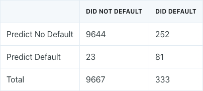
The confusion matrix shows that out of the 333 individuals who defaulted, 252 were missed by linear discriminant analysis, which is a 75.7% error rate. This is known as a class-specific error rate.

Linear discriminant analysis does a poor job of classifying customers who default because it is trying to approximate the Bayes’ classifier, which has the lowest total error rate instead of class-specific error rate.

The probability threshold for determining defaults could be lowered to improve the model. Lowering the probability threshold to 20% results in the following confusion matrix:

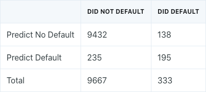
Now, linear discriminant analysis correctly predicts 195 individuals who defaulted, out of the 333 total. This is an improvement over the previous error rate. However, 235 individuals who do not default are classified as defaulters, compared to only 23 previously. This is the tradeoff that results from lowering the probability threshold.

The threshold value to use in a real situation should be based on domain and industry knowledge, such as information about the costs associated with defaults.

ROC Curve

The ROC curve is a popular graphic for simultaneously displaying the two types of errors for all possible thresholds.

The overall performance of a classifier summarized over all possible thresholds is given by the area under the curve (AUC). An ideal ROC curve will hug the top left corner, so the larger the AUC, the better the classifier. A classifier that performs no better than chance will have an AUC of 0.50.

Below is an example of an ideal ROC curve (blue) versus an ROC curve that indicates that the model performs no better than chance (black).

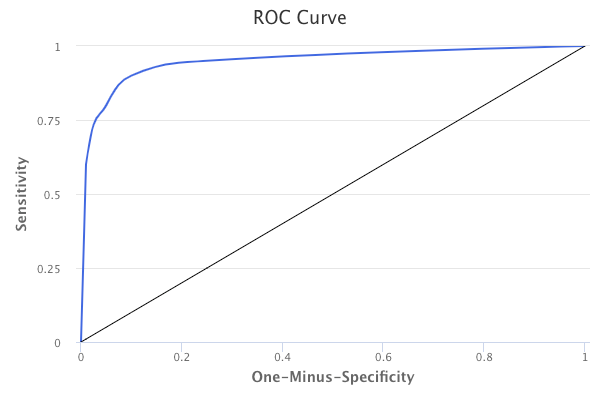
ROC curves are useful for comparing different classifiers because they account for all possible probability threshold values.

The Y axis indicates the True Positive Rate, which is also known as the sensitivity. In the context of the Credit Default data, it represents the fraction of defaulters who are correctly classified.

The X axis indicates the False Positive Rate, which is also known as the one-minus-specificity. In the context of the Credit Default data, it represents the fraction of non-defaulters who are incorrectly classified.

The ROC curve is very useful in comparing different classification models for the same dataset because it accounts for all possible threshold values. If the AUC of one model is much better than the others, it is the best model to use.

Quadratic Discriminant Analysis

Linear discriminant analysis assumes that observations within each class are drawn from a multivariate normal distribution with class-specific means and a common covariance matrix for all of the classes.

Quadratic discriminant analysis assumes that each class has its own covariance matrix. In other words, quadratic discriminant analysis relaxes the assumption of the common covariance matrix.

Linear vs Quadratic Discriminant Analysis

Which method is better for classification? LDA or QDA? The answer lies in the bias-variance tradeoff.

LDA is a less flexible classifier, meaning it has lower variance than QDA. However, if the assumption of the common covariance matrix is badly off, then LDA could suffer from high bias.

In general, LDA tends to be a better classifier than QDA if there are relatively few observations in the training data because reducing variance is crucial in this case.

In general, QDA is recommended over LDA if the training data is large, meaning that the variance of the classifier is not a major concern. QDA is also recommended over LDA if the assumption of the common covariance matrix is flawed.

K-Nearest Neighbors

K-Nearest Neighbors (KNN) is a popular nonparametric classifier method.

Given a positive integer K and some test observation, the KNN classifier identifies the K points in the training data that are closest to the test observation. These closest K points are represented by N₀. Then, it estimates the conditional probability for a class as the fraction of points in N₀ that represent that specific class. Lastly, KNN will apply the Bayes’ rule and classify the test observation to the class with the largest probability.

However, the choice of the K value is very important. Lower values are more flexible, whereas higher values are less flexible but have more bias. Similar to the regression setting, a bias-variance tradeoff exists.

Comparison of Classification Methods

There are four main classification methods: logistic regression, LDA, QDA, and KNN.

Logistic regression and LDA are closely connected. They both produce linear decision boundaries. However, LDA may provide improvement over logistic regression when the assumption of the normal distribution with common covariance for classes holds. Additionally, LDA may be better when the classes are well separated. On the other hand, logistic regression outperforms LDA when the normal distribution assumption is not met.

KNN is a completely non-parametric approach. There are no assumptions made about the shape of the decision boundary. KNN will outperform both logistic regression and LDA when the decision boundary is highly nonlinear. However, KNN does not indicate which predictors are important.

QDA serves as a compromise between the nonparametric KNN method and the linear LDA and logistic regression methods.

Originally published at https://www.bijenpatel.com on August 4, 2020.

I will be releasing the equivalent Python code for these examples soon. Subscribe to get notified!

ISLR Chapter 4 — R Code

Logistic Regression

library(MASS) # For model functions
library(ISLR) # For datasets
library(ggplot2) # For plotting
library(dplyr) # For easy data manipulation functions
library(caret) # For confusion matrix function
library(e1071) # Requirement for caret library

# Working with the Stock Market dataset to predict direction of stock market movement (up/down)
head(Smarket)
summary(Smarket)

# Fit a logistic regression model to the data
# The direction of the stock market is the response
# The lags (% change in market on previous day, 2 days ago, etc.) and trade volume are the predictors
Smarket_logistic_1 = glm(Direction ~ Lag1 + Lag2 + Lag3 + Lag4 + Lag5 + Volume, family="binomial", data=Smarket)

summary(Smarket_logistic_1)

# Use the contrasts function to determine which direction is indicated as "1"
contrasts(Smarket$Direction)
##      Up
## Down  0
## Up    1

# Use the names function to determine the objects in the logistic model
names(Smarket_logistic_1)

# Get confusion matrix to determine accuracy of the logistic model
Smarket_predictions_1 = data.frame(Direction=Smarket_logistic_1$fitted.values)</span><span id="f484" class="de ke ii ef ly b db mc md me mf mg ma w mb">Smarket_predictions_1 = mutate(Smarket_predictions_1, Direction = ifelse(Direction >= 0.50, "Up", "Down")</span><span id="9340" class="de ke ii ef ly b db mc md me mf mg ma w mb">Smarket_predictions_1$Direction = factor(Smarket_predictions_1$Direction, levels=c("Down", "Up"), ordered=TRUE)</span><span id="bf0d" class="de ke ii ef ly b db mc md me mf mg ma w mb">confusionMatrix(Smarket_predictions_1$Direction, Smarket$Direction, positive="Up")

# Instead of fitting logistic model to the entire data, split the data into training/test sets
Smarket_train = filter(Smarket, Year <= 2004)
Smarket_test = filter(Smarket, Year == 2005)

Smarket_logistic_2 = glm(Direction ~ Lag1 + Lag2 + Lag3 + Lag4 + Lag5 + Volume, family="binomial", data=Smarket_train)

# Use the model to make predictions on the test data
Smarket_test_predictions = predict(Smarket_logistic_2, Smarket_test, type="response")

# Get confusion matrix to determine accuracy on the test dataset
Smarket_test_predictions = data.frame(Direction=Smarket_test_predictions)</span><span id="e401" class="de ke ii ef ly b db mc md me mf mg ma w mb">Smarket_test_predictions = mutate(Smarket_test_predictions, Direction = ifelse(Direction >= 0.50, "Up", "Down"))</span><span id="57f9" class="de ke ii ef ly b db mc md me mf mg ma w mb">Smarket_test_predictions$Direction = factor(Smarket_test_predictions$Direction, levels=c("Down", "Up"), ordered=TRUE)</span><span id="5c57" class="de ke ii ef ly b db mc md me mf mg ma w mb">confusionMatrix(Smarket_test_predictions$Direction, Smarket_test$Direction)

# Fit a better logistic model that only considers the most important predictors (Lag1, Lag2)
Smarket_logistic_3 = glm(Direction ~ Lag1 + Lag2, family="binomial", data=Smarket_train)

# Repeat the procedure to obtain a confusion matrix for the test data ...</span>

Linear Discriminant Analysis

# Continuing to work with the Stock Market dataset

# The lda function is used to fit a linear discriminant model
Smarket_lda = lda(Direction ~ Lag1 + Lag2, data=Smarket_train)
Smarket_lda # View the prior probabilities, group means, and coefficients

# Plot of the linear discriminants of each observation in the training data, separated by class
plot(Smarket_lda)

# Use the model to make predictions on the test dataset
Smarket_lda_predictions = predict(Smarket_lda, Smarket_test)

# View the confusion matrix to assess accuracy
confusionMatrix(Smarket_lda_predictions$class, Smarket_test$Direction, positive="Up")

# Notice that a predicted probability >= 50% actually corresponds to "Down" in LDA
Smarket_lda_predictions$posterior[1:20]
Smarket_lda_predictions$class[1:20]</span>

Quadratic Discriminant Analysis

# Continue to work with the Stock Market dataset

# The qda function is used to fit a quadratic discriminant model
Smarket_qda = qda(Direction ~ Lag1 + Lag2, data=Smarket_train)
Smarket_qda # View the prior probabilities and group means

# Use the model to make predictions on the test dataset
Smarket_qda_predictions = predict(Smarket_qda, Smarket_test)

# View the confusion matrix to assess accuracy
confusionMatrix(Smarket_qda_predictions$class, Smarket_test$Direction, positive="Up")

# Notice that a predicted probability >= 50% actually corresponds to "Down" in QDA
Smarket_qda_predictions$posterior[1:20]
Smarket_qda_predictions$class[1:20]</span>

KNN

# Continue to work with the Stock Market dataset
library(class) # The class library is used for KNN

# Before performing KNN, separate dataframes are made for the predictors and responses
Smarket_train_predictors = data.frame(Lag1=Smarket_train$Lag1, Lag2=Smarket_train$Lag2)
Smarket_test_predictors = data.frame(Lag1=Smarket_test$Lag1, Lag2=Smarket_test$Lag2)
Smarket_train_response = Smarket_train$Direction
Smarket_test_response = Smarket_test$Direction

# Perform KNN with K=3
set.seed(1)

Smarket_predictions_knn = knn(Smarket_train_predictors,
                            Smarket_test_predictors,
                            Smarket_train_response,
                            k=3)

# See a confusion matrix to assess the accuracy of KNN
confusionMatrix(Smarket_predictions_knn, Smarket_test_response)

# Next, we will use KNN on the Caravan data to predict whether or not someone will purchase caravan insurance
# The data contains demographic data on individuals, and whether or not insurance was bought

# Before performing KNN, predictors should be scaled to have mean 0 and standard deviation 1
Caravan_scaled = scale(Caravan[,-86])

# We will designate the first 1000 rows as the test data and the remaining as training data
# Create separate datasets for the predictors and responses
Caravan_test_predictors = Caravan_scaled[1:1000,]
Caravan_train_predictors = Caravan_scaled[1001:5822,]
Caravan_test_response = Caravan[1:1000, 86]
Caravan_train_response = Caravan[1001:5822, 86]

# Perform KNN
set.seed(1)
Caravan_knn_predictions = knn(Caravan_train_predictors,
                            Caravan_test_predictors,
                            Caravan_train_response,
                            k=5)

# Assess accuracy
confusionMatrix(Caravan_knn_predictions, Caravan_test_response, positive="Yes")
    # 26.67% accuracy is better than 6% from random guessing</span>