This is a summary of chapter 5 of the Introduction to Statistical Learning textbook. I’ve written a 10-part guide that covers the entire book. The guide can be read at my website, or here at Hashnode. Subscribe to stay up to date on my latest Data Science & Engineering guides!
Resampling methods involve repeatedly drawing samples from a training dataset and refitting a statistical model on each of the samples in order to obtain additional information about the fitted model.
For example, to estimate the variability of a linear regression model, we can repeatedly draw different samples from the training data, fit a linear regression model to each new sample, and then examine the extent to which the fits differ.
There are two resampling methods that are most common:
Cross validation can be used to estimate the test error of a specific statistical learning method, or to select the appropriate level of flexibility of a method.
Bootstrap can be used to help provide the accuracy of parameter estimates, or of a statistical learning method.
Cross-Validation
There is a difference between the training error and the test error. The test error is what we are much more interested in measuring. However, we do not always have a large test dataset available to estimate the test error.
Many techniques exist to estimate the test error with the training data. These techniques fall into one of two categories:
- Applying a mathematical adjustment to the training error
- Holding out a subset of the training data from the fitting process and applying the model to the held-out data
Validation Set Approach
The Validation Set Approach is a simple strategy for estimating the test error.
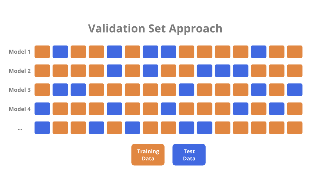
The available training data is randomly divided into a training set and test (hold-out) set. A model is fit to the training set, and is used to make predictions on the data in the test set. The error from the predictions on the test set serves as the estimate for the test error.
In regression, the measure of error is usually the Mean Squared Error (MSE). In classification, the measure of error is usually the misclassification rate.
To be sure about which model to fit, the Validation Set Approach process could be repeated multiple times to allow for differences in random data assignment between the training and test sets.

There are two drawbacks associated with the Validation Set Approach:
- The validation estimate of the test error can be highly variable, depending on precisely which observations are randomly assigned to the training set and test set.
- Since only a subset of the observations are used to fit the model, the validation set error may overestimate the test error because statistical methods tend to perform worse when trained on fewer observations.
Cross-validation is a refinement to the Validation Set Approach that addresses these drawbacks.
Leave-One-Out Cross-Validation (LOOCV)
Leave-One-Out Cross-Validation (LOOCV) is closely related to the Validation Set Approach, but attempts to address the drawbacks.
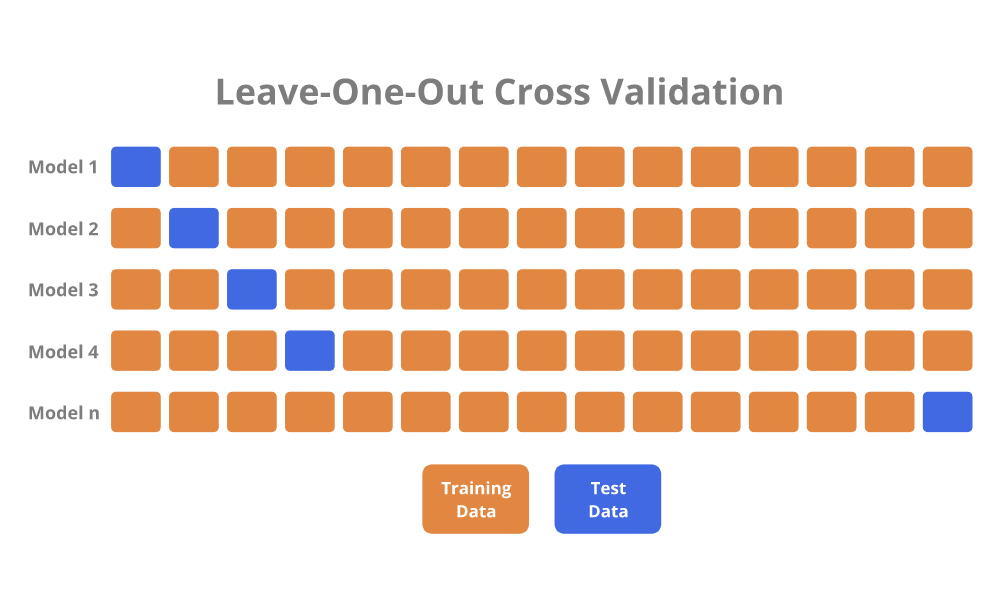
Similar to the Validation Set Approach, LOOCV involves splitting a full dataset into separate training and test sets. However, only a single observation is included in the test set, and all of the remaining observations are assigned to the training set.
A model is fit to the training set, and a prediction is made for the single excluded observation in the test set. The test error is determined for the prediction. Then, the LOOCV procedure is repeated to individually exclude each observation from the full dataset. Finally, the LOOCV estimate for the test error is simply the average of all of the individual test errors.

LOOCV has two advantages over the Validation Set Approach:
- LOOCV is not highly variable because it will yield identical results each time it is performed.
- LOOCV has far less bias because almost the entire dataset is being used to fit a model. Therefore, LOOCV does not overestimate the test error as much as the Validation Set Approach.
However, LOOCV has one potentially major disadvantage:
K-Fold Cross-Validation
K-Fold Cross-Validation (K-Fold CV) is an alternative to LOOCV, and is typically the preferred method.
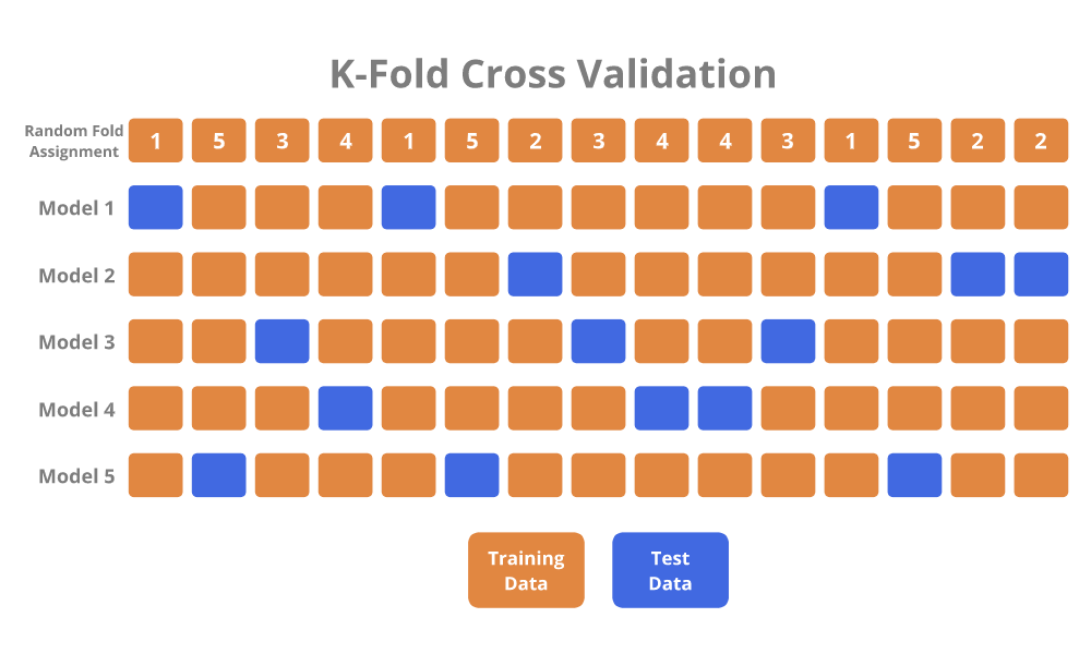
It involves randomly dividing observations into K groups (folds) of approximately the same size.
The first fold is treated as the test set, and a model is fit to the remaining folds. The fitted model is used to make predictions on the observations in the first fold, and the test error is measured. The K-Fold CV procedure is repeated K times so that a different fold is treated as the test set each time. Finally, the K-Fold CV estimate of the test error is simply the average of the K test measures.

LOOCV is basically a special case of K-Fold CV, in which K is set equal to n.
K-Fold CV has two advantages over LOOCV:
- K-Fold CV is much less computationally expensive.
- K-Fold CV is advantangeous when it comes to the Bias-Variance tradeoff.
The K-Fold CV test error estimates have a lower variance than the LOOCV estimates because more observations are included in the test set. Overall, K-Fold CV provides a more accurate measure of the test error.
Typically, K = 5 or K = 10 is chosen for K-Fold CV because these have been shown to empirically yield test error estimates that suffer neither from excessively high bias nor variance.
Bootstrap
The bootstrap is a widely acceptable and extremely powerful statistical tool that can be used to quantify the uncertainty associated with an estimator or statistical learning method.
The point of the bootstrap can be illustrated with an example where we are trying to figure out the best investment allocation under a simple model.
Assume that we want to invest $10,000 into two stocks that yield X and Y, respectively:
- Stock A: X Return (random quantity)
- Stock B: Y Return (random quantity)
- Stock A and Stock B are not the same, and have different means and variances for their returns
We will invest α into A, and 1-α into B. Additionally, α will be chosen to minimize the total risk of investment since there is variability associated with the returns. The equation to determine the α value that minimizes risk is as follows:

The variances are unknown, but could be estimated through past data of returns for the investments. Plugging the variances into the equation would let us know the value for α.
However, since we only have one dataset, we can only determine one value for α. But what if we wanted to estimate the accuracy of the estimate for α? To estimate a variance for the α value itself, we would need hundreds of datasets. However, we usually cannot simply generate new samples from the original population. The bootstrap approach allows us to emulate the process of obtaining new sample datasets so that we can estimate variability without actually generating new sample datasets. Instead of obtaining new independent datasets from the population, the bootstrap method obtains distinct datasets by repeatedly sampling observations from the original dataset.

For example, assume that we have a dataset of 15 observations for the returns of A and B. The bootstrap method randomly selects 15 observations from the dataset to produce a new bootstrapped dataset. The selection is done with replacement, meaning that it is possible for the same observation to occur more than one time in the bootstrapped dataset. The bootstrapping procedure is repeated a large number of times (usually 1000) so that 1000 bootstrapped datasets are generated. These datasets would give us 1000 values for α, which would help us ultimately determine the variance for α.
Originally published at https://www.bijenpatel.com on August 5, 2020.
I will be releasing the equivalent Python code for these examples soon. Subscribe to get notified!
ISLR Chapter 5 — R Code
Validation Set Approach
library(ISLR)
library(MASS)
library(ggplot2)
library(dplyr)

# We will work with the Auto dataset
head(Auto)

# The set.seed function allows reproducibility of results any time that random numbers are being generated
# It takes an arbitrary integer value
set.seed(1)

# The Validation Set approach involves randomly splitting the data into two halves
nrow(Auto) # Determine how many rows of data we have
train = sample(392, 196) # Randomly choose which 196 rows to use for the training data
Auto_train = Auto[train,] # Create a training set
Auto_test = Auto[-train,] # Create a test set

# Fit a simple linear model to the training data
# We are attempting to predict a vehicle's Miles per Gallon with Horsepower as the predictor
Auto_lm_1 = lm(mpg ~ horsepower, data=Auto_train)

# Use the fitted model to predict on the held-out test data
Auto_test_predictions = predict(Auto_lm_1, Auto_test)

# Determine the Mean Squared Error (MSE) of the test data, which is a measure of the test error
Auto_test_mse = data.frame(mpg=Auto_test$mpg, predicted_mpg=Auto_test_predictions)
Auto_test_mse$sq_error = (Auto_test_mse$mpg - Auto_test_mse$predicted_mpg)^2
Auto_lm_1_mse = mean(Auto_test_mse$sq_error)

# Fit a polynomial regression model instead, which seems to be a better choice
Auto_lm_2 = lm(mpg ~ horsepower + I(horsepower^2), data=Auto_train)
Auto_test_predictions_2 = predict(Auto_lm_2, Auto_test)
Auto_test_mse_2 = data.frame(mpg=Auto_test$mpg, predicted_mpg=Auto_test_predictions_2)
Auto_test_mse_2$sq_error = (Auto_test_mse_2$mpg - Auto_test_mse_2$predicted_mpg)^2
Auto_lm_2_mse = mean(Auto_test_mse_2$sq_error)

# Running same models with different random training/test splits results in different errors
set.seed(2)
train = sample(392, 196)
# Repeat above models to see that MSE will be slightly different
# This is because variance increases due to only using half the data to fit the model</span>
Leave-One-Out Cross Validation
library(boot) # For the cv.glm function

# We continue working with the Auto data

# We use the glm function instead of the lm function to fit a linear regression model
# This is because a glm object can be used with the cv.glm function from the boot library
# We fit the model to the entire Auto data because cv.glm will perform the LOOCV for us
Auto_glm_1 = glm(mpg ~ horsepower, data=Auto)

# Perform LOOCV and determine the test error
Auto_glm_1_cv = cv.glm(data=Auto, glmfit=Auto_glm_1) # Perform LOOCV
Auto_glm_1_cv$delta # Test error is stored in the delta component
# There are two values
# The first value is the standard CV estimate
# The second value is a bias-corrected CV estimate

# What if we wanted to get LOOCV test error estimates for five different polynomial models?
# Easily fit five different polynomial models from degree 1 to 5 and compare their test errors
Auto_loocv_errors = rep(0, 5) # Create initial vector for the errors</span><span id="c3a1" class="de kv ii ef lp b db lt lu lv lw lx lr w ls"># The for loop goes through all five degrees and stores their errors
for (i in 1:5){
    Auto_glm = glm(mpg ~ poly(horsepower, i), data=Auto)
    Auto_loocv_errors[i] = cv.glm(data=Auto, glmfit=Auto_glm)$delta[1]
    }

# Plot the different model degrees and their errors with ggplot
Auto_loocv_errors = data.frame(Degree = c(1, 2, 3, 4, 5), Error = Auto_loocv_errors)

Auto_loocv_errors_plot = ggplot(Auto_loocv_errors, aes(x=Degree, y=Error)) +
    geom_line() +
    labs(title="Auto LOOCV Errors", subtitle="Polynomial Models (Degrees 1 to 5)", x="Degree", y="LOOCV Error") +
    geom_line(colour="red")

plot(Auto_loocv_errors_plot)</span>
K-Fold Cross Validation
# What if we wanted K-Fold test error estimates instead of LOOCV?
# We can easily repurpose the previous for loop for K-Fold CV
# We will perform 10-Fold CV on the Auto data
Auto_tenfold_errors = rep(0, 5) # Create initial vector for the errors

for (i in 1:5){
    Auto_glm = glm(mpg ~ poly(horsepower, i), data=Auto)
    Auto_tenfold_errors[i] = cv.glm(data=Auto, glmfit=Auto_glm, K=10)$delta[1]
    }
    # Simply change the previous for loop by adding K=10

# Plot the different model degrees and their K-Fold errors with ggplot
Auto_tenfold_errors = data.frame(Degree = c(1, 2, 3, 4, 5), Error = Auto_tenfold_errors)

Auto_tenfold_errors_plot = ggplot(Auto_tenfold_errors, aes(x=Degree, y=Error)) +
    geom_line() +
    labs(title="Auto 10-Fold Errors", subtitle="Polynomial Models (Degrees 1 to 5)", x="Degree", y="10-Fold Error") +
    geom_line(colour="red")

plot(Auto_tenfold_errors_plot)</span>
Bootstrap
library(boot) # The boot library is also for bootstrap

# Bootstrap can be used to assess the variability of coefficient estimates of a model

# First, we create a simple function to get coefficient values from a linear regression model
coef_function = function(data, index)
    return(lm(mpg ~ horsepower + I(horsepower^2), data=data, subset=index)$coefficients)

# Test the function by fitting a linear model to the entire Auto dataset
coef_function(Auto, 1:392)
# We specified data=Auto and index=1:392

# Now, we test the function with a dataset through the bootstrap resampling method
# Bootstrap creates a new dataset by randomly sampling from the original data WITH replacement
set.seed(1)
coef_function(Auto, sample(392, 392, replace=T)

# So far, that was only one result from one bootstrap dataset
# What if we wanted to get 1000 results?
# Use the boot function to get 1000 bootstrap estimates for the coefficients and standard errors
boot(Auto, coef_function, 1000)

# Compare results of the bootstrap estimates to the standard quadratic model on the original data
summary(lm(mpg ~ horsepower + I(horsepower^2), data=Auto))$coef</span>
