This is a summary of chapter 6 of the Introduction to Statistical Learning textbook. I’ve written a 10-part guide that covers the entire book. The guide can be read at my website, or here at Hashnode. Subscribe to stay up to date on my latest Data Science & Engineering guides!

Linear regression can be improved by replacing plain least squares with some alternative fitting procedures. These alternative fitting procedures may yield better prediction accuracy and model interpretability.

Alternative Methods

There are three classes of alternative methods to least squares: subset selection, shrinkage, and dimension reduction.

Subset Selection

Subset selection involves identifying a subset of the p predictors that are believed to be related to the response, and fitting a least squares model to the reduced set of predictors.

Shrinkage

Shrinkage involves fitting a model involving all p predictors. However, the estimated coefficients are shrunken towards zero relative to the least squares estimates. Shrinkage reduces variance, and may perform variable selection.

Dimension Reduction

Dimension reduction involves projecting all of the p predictors into an M-dimensional subspace where M<p. M different “linear combinations” of all of the p predictors are computed, and are used as predictors to fit a linear regression model through least squares.

Improved Prediction Accuracy

When the number of observations n is not much greater than the number of predictors p, least squares regression will tend to have higher variance. In the case that the number of predictors p is greater than the number of observations n, least squares cannot be used at all.

By shrinking or constraining the estimated coefficients through alternative methods, variance can be substantially reduced at a negligible increase to bias.

Improved Model Interpretability

Additionally, the least squares approach is highly unlikely to yield any coefficient estimates that are exactly zero. There are alternative approaches that automatically perform feature selection for excluding irrelevant variables from a linear regression model, thus resulting in a model that is easier to interpret.

Subset Selection

There are two main types of subset selection methods: best subset selection and stepwise model selection.

Best Subset Selection

Best subset selection involves fitting a separate least squares regression model for each possible combination of the p predictors. For example, assume we had a credit balance dataset that looked like the following:

The best subset selection process begins by fitting all models that contain only one predictor:

Next, all possible two-predictor models are fit:

The process is continued for all possible three, four, and five predictor models.

After all possible models are fit, the best one, two, three, four, and five predictor models are chosen based on some criteria, such as the largest R² value. For the credit balance dataset, these models may be as follows:

Lastly, the overall best model is chosen from the remaining models. The best model is chosen through cross-validation or some other method that chooses the model with the lowest measure of test error. In this final step, a model cannot be chosen based on R², because R² always increases when more predictors are added. The plot of the K-Fold CV test errors for the five models looks as follows:

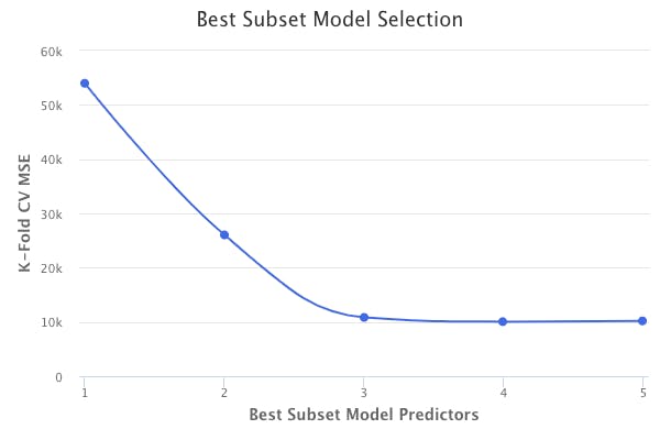
The model with four predictors has the lowest test error, and thus would be chosen as the best overall model.

Stepwise Selection

There are three different types of stepwise selection: forward, backward, and hybrid. Compared to best subset selection, stepwise selection is computationally more feasible. Additionally, it helps avoid the issue of overfitting and high variance.

Forward Stepwise Selection

Forward stepwise selection begins with a model containing no predictors. Predictors are added to the model one at a time, based on the predictor that gives the greatest additional improvement to the fit of the model.

After using forward stepwise selection to come up with the best one, two, three, four, and five predictor models, cross-validation is used to choose the best model.

The disadvantage to forward stepwise selection is that the method does not guarantee to find the best possible model, since the final model is dependent on the first predictor that is added to the null model. The credit balance dataset is a good example of this phenomenon. Best subset selection and forward stepwise selection both choose the same one-, two-, and three-predictor models. However, they differ in the fourth model.

Best subset selection replaces the “Rating” predictor with the “Cards” predictor.

Since forward stepwise selection begins by choosing “Rating” as the first predictor, the predictor is kept:

Backward Stepwise Selection

Backward stepwise selection begins with a model that contains all of the predictors. Predictors are removed from the model one at a time, based on the predictor that is least useful towards the fit of the model.

After using backward stepwise selection to come up with the best one, two, three, and four predictor models, cross-validation is used to choose the best model.

Backward stepwise selection has the same disadvantage as forward stepwise selection in that it is not guaranteed to find the best possible model.

Hybrid Stepwise Selection

Hybrid stepwise selection is a combination of forward and backward selection. We begin with a null model that contains no predictors. Then, variables are added one by one, exactly as done in forward selection. However, if at any point the p-value for some variable rises above a chosen threshold, then it is removed from the model, as done in backward selection.

Optimal Model Selection

In order to select the best model with respect to the test error, the test error needs to be estimated through one of two methods:

1. An indirect estimate through some kind of mathematical adjustment to the training error, which accounts for bias due to overfitting.
2. A direct estimate through a method such as cross-validation.

Indirect Estimation of Test Error

There are various different methods of indirectly estimating the test error: Cp, AIC, BIC, and adjusted-R².

Cp

Cp is an estimate of test error that adds a penalty to the training error, based on the number of predictors and the estimate of the variance of error. The model with the lowest Cp is chosen as the best model.

AIC

Similar to Cp, AIC is another estimate of test error that adds a penalty to the training error, based on the number of predictors and the estimate of the variance of error. However, it is defined for a larger class of models fit by maximum likelihood. The model with the lowest AIC is chosen as the best model.

BIC

BIC is an estimate of test error that is similar to AIC, but places a heavier penalty on models with a large number of predictors. Therefore, BIC results in the selection of models with less predictors. The model with the lowest BIC is chosen as the best model.

Adjusted-R²

Adjusted-R² is a measure that penalizes the R² value for the inclusion of unnecessary predictors. The model with the highest adjusted-R² is chosen as the best model.

One-Standard-Error Rule

The model with the absolute lowest test error doesn’t always have to be chosen. For example, what if we had a case where the models with anywhere from 3 to 10 predictors all had similar test errors?

A model could be chosen based on the one-standard-error rule. This rule involves selecting the model with the least number of predictors for which the estimated test error is within one standard error of the model with the absolute minimum error. This is done for simplicity and ease of interpretability.

Shrinkage Methods

Shrinkage methods involve fitting a model with all of the available predictors, and shrinking the coefficients towards zero. There are two main shrinkage methods:

1. Ridge Regression
2. Lasso Regression

Ridge Regression

Recall that least squares regression minimizes RSS to estimate coefficients. The coefficients are unbiased, meaning that least squares doesn’t take variable significance into consideration when determining the coefficient values.

Instead, ridge regression minimizes the following:

The second term is called a shrinkage penalty, and is the term that shrinks the coefficient estimates towards zero. λ is a tuning parameter that controls the relative impact of the penalty term on the regression model. The coefficient estimates that come from ridge regression are biased because variable significance is taken into consideration.

Performing ridge regression with different values of λ on the credit balance dataset would result in the following sets of standardized coefficients:

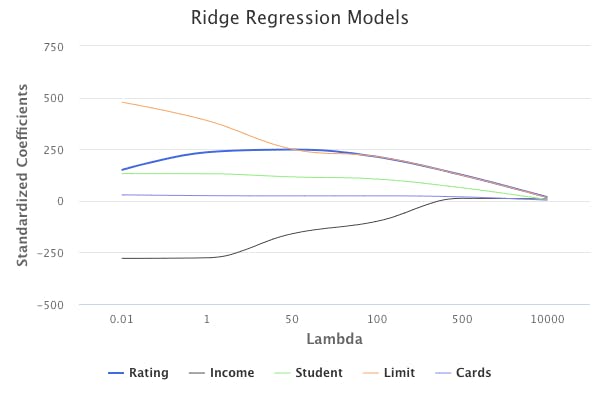
In short, different values of λ will produce different sets of coefficient estimates. Therefore, choosing the proper λ value is critical, and is usually chosen through cross-validation.

Additionally, in ridge regression, coefficient estimates significantly depend on the scaling of predictors. Therefore, it is best practice to perform ridge regression after standardizing the predictors, so that they are on the same scale.

Ridge Regression vs Least Squares Regression

So, when is it appropriate to use ridge regression over least squares regression?

The advantage of ridge regression is rooted in the bias-variance tradeoff. As λ increases, the flexibility of the ridge regression model decreases, resulting in a decrease in variance, but an increase in bias.

Therefore, ridge regression should be used when least squares regression will have high variance. This happens when the number of predictors is almost as large as the number of observations.

If we’re unsure whether or not ridge regression would result in a better predictive model than least squares, we could simply run both methods and compare the test errors to each other. Unless ridge regression provides a significant advantage, least squares should be used for model simplicity and interpretability.

Lasso Regression

The disadvantage of ridge regression is that all predictors are included in the final model. Even though the penalty term shrinks the coefficient estimates towards zero, it does not set them to exactly zero.

This might not matter in terms of prediction accuracy, but it creates a challenge when it comes to model interpretation because of the large number of predictors.

Lasso regression is an alternative to ridge regression, which overcomes this disadvantage. Lasso regression minimizes the following:

Similar to ridge regression, lasso regression will shrink coefficient estimates towards zero. However, the penalty is a bit different in that it forces some of the coefficient estimates to be exactly zero when the tuning parameter λ is large enough. Again, choosing the appropriate λ value is critical.

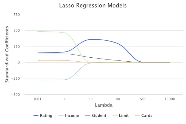
This effectively means that lasso regression performs variable selection, and makes it easier to interpret the final model.

As in ridge regression, it is best practice to perform lasso regression after standardizing the predictors.

Ridge Regression vs Lasso Regression

In general, lasso regression is expected to perform better than ridge regression when the response Y is expected to be a function of only a few of the predictors.

In general, ridge regression is expected to perform better than lasso regression when the response is expected to be a function of a large number of predictors.

Cross-validation should be used to compare both methods and choose the best model.

Selecting the Tuning Parameter λ

As mentioned previously, choosing the proper value for the tuning parameter is crucial for coming up with the best model.

Cross-validation is a simple method of choosing the appropriate λ value. First, create a grid of different λ values, and determine the cross-validation test error for each value. Finally, choose the value that resulted in the lowest error.

Dimension Reduction Methods

When we have a dataset with a large number of predictors, dimension reduction methods can be used to summarize the dataset with a smaller number of representative predictors (dimensions) that collectively explain most of the variability in the data. Each of the dimensions is some linear combination of all of the predictors. For example, if we had a dataset of 5 predictors, the first dimension Z₁ would be as follows:

And a final regression model might look as follows:

Note that we will always have less dimensions than the number of predictors.

The ϕ values for the dimensions are known as loading values. The values are subject to the constraint that the square of the ϕ values in a dimension must equal one. For our above example, this means that:

The ϕ values in a dimension make up a “loading vector” that defines a “direction” to explain the predictors. But how exactly do we come up with the ϕ values? They are determined through either of the two most common dimension reduction methods:

1. Principal Components Analysis
2. Partial Least Squares

Principal Components Analysis

Principal components analysis is the most popular dimension reduction method. The method involves determining different principal component directions of the data.

The first principal component direction Z₁ defines the direction along which the data varies the most. In other words, it is a linear combination of all of the predictors, such that it explains most of the variance in the predictors.

The second principal component direction Z₂ defines another direction along which the data varies the most, but is subject to the constraint that it must be uncorrelated with the first principal component, Z₁.

The third principal component direction Z₃ defines another direction along which the data varies the most, but is subject to the constraint that it must be uncorrelated with both of the previous principal components, Z₁ and Z₂.

And so on and so forth for additional principal component directions.

Dimension reduction is best explained with an example. Assume that we have a dataset of different baseball players, which consists of their statistics in 1986, their years in the league, and their salaries in the following year (1987).

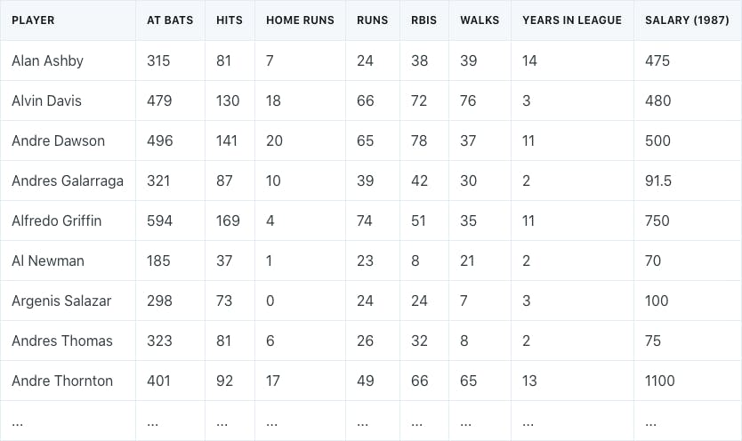
Our goal is to perform principal components regression to come up with a model that predicts salaries.

First, we need to perform dimension reduction by transforming our 7 different predictors into a smaller number of principal components to use for regression.

It is important to note that prior to performing principal components analysis, each predictor should be standardized to ensure that all of the predictors are on the same scale. The absence of standardization will cause the predictors with high variance to play a larger role in the final principal components obtained.

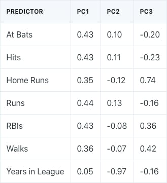
Performing principal components analysis would result in the following ϕ values for the first three principal components:

A plot of the loading values of the first two principal components would look as follows:

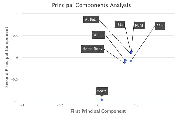
How do we interpret these principal components?

If we take a look at the first principal component, we can see that there is approximately an equal weight placed on each of the six baseball statistic predictors, and much less weight placed on the years that a player has been in the league. This means that the first principal component roughly corresponds to a player’s level of production.

On the other hand, in the second principal component, we can see that there is a large weight placed on the number of years that a player has been in the league, and much less weight placed on the baseball statistics. This means that the second principal component roughly corresponds to how long a player has been in the league.

In the third principal component, we can see that there is more weight placed on three specific baseball statistics: home runs, RBIs, and walks. This means that the third principal component roughly corresponds to a player’s batting ability.

Performing principal components analysis also tells us the percent of variation in the data that is explained by each of the components. The first principal component from the baseball data explains 67% of the variation in the predictors. The second principal component explains 15%. The third principal component explains 9%. Therefore, together, these three principal components explain 91% of the variation in the data.

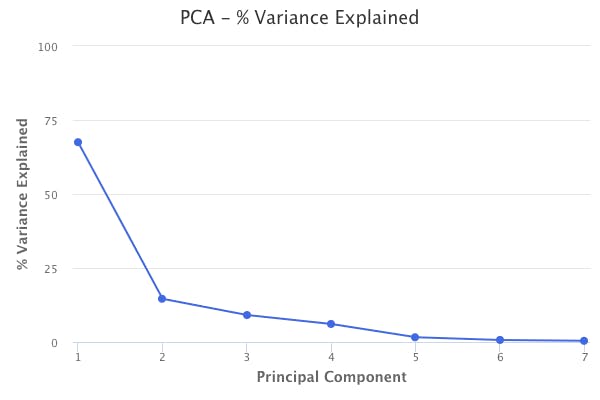
This helps explain the key idea of principal components analysis, which is that a small number of principal components are sufficient to explain most of the variability in the data. Through principal components analysis, we’ve reduced the dimensions of our dataset from seven to three.

The number of principal components to use in regression can be chosen in one of two ways. The first method involves simply using the number of components that explain a large amount of the variation in the data. For example, in the baseball data, the first three principal components explain 91% of variation in the data, so using just the first three is a valid option. The second method involves choosing the number of principal components that results in the regression model with the lowest test error. Typically, both methods should result in the same or similar final models with test errors that do not greatly differ from one another.

Principal Components Regression vs Least Squares Regression

Remember that in principal components analysis, the response variable is not used to determine the principal components. Therefore, in principal components regression, we are making the assumption that the directions in which the predictors show the most variation are also the directions that are associated with the response variable.

The assumption is not guaranteed to be true, but it often turns out to be a reasonable assumption to make. When the assumption holds, principal components regression will result in a better model than least squares regression due to mitigation of overfitting.

In general, principal components regression will perform well when the first few principal components are sufficient to capture most of the variation in the predictors, as well as the relationship with the response variable.

However, principal components regression is not a feature selection method because each of the principal components is a linear combination of all of original predictors in the dataset. If performing feature selection is important, then another method such as stepwise selection or lasso regression should be used.

Partial Least Squares Regression

In principal components regression, the directions that best represent the predictors are identified in an unsupervised way since the response variable is not used to help determine the directions. Therefore, there is no guarantee that the directions that best explain the predictors will also be the best directions to use for predicting the response.

Partial least squares regression is a supervised alternative to principal components regression. In other words, partial least squares regression attempts to find directions that help explain both the response and the predictors.

Partial least squares works by first standardizing the predictors and response, and then determining the first direction by setting each ϕ value equal to the coefficients from simple linear regression of the response onto each of the predictors. In doing so, partial least squares places the highest weight on the variables most strongly related to the response.

To identify the second direction, each of the original variables is adjusted by regressing each variable onto the first direction and taking the residuals. These residuals represent the remaining information that isn’t explained by the first direction. The second direction is then determined by using the new residual data, in the same method that the first direction was determined based on the original data. This iterative approach is repeated to find multiple directions, which are then used to fit a linear model to predict the response.

The number of directions to use in partial least squares regression should be determined through cross-validation.

However, partial least squares regression usually does not perform better than ridge regression or principal components regression. This is because supervised dimension reduction can reduce bias, but also has the potential to increase variance.

Considerations in High Dimensions

Today, it is common to be able to collect hundreds or even thousands of predictors for our data. The high dimensional setting refers to situations where the number of predictors exceeds the number of observations we have available. In the high dimensional setting, least squares cannot be used because it will result in coefficient estimates that are a perfect fit to the data, such that the residuals are zero. This is where subset selection, ridge regression, lasso, principal components regression, and partial least squares should be used instead.

However, the interpretation of model results is a bit different. For example, assume that we are trying to predict blood pressure from hundreds of predictors. A forward stepwise selection model might indicate that 20 of the predictors lead to a good predictive model. It would actually be improper to conclude that these 20 predictors are the best to predict blood pressure. Since we have hundreds of predictors, a different dataset might actually result in a totally different predictive model. Therefore, we must indicate that we have identified one of the many possible models, and it must be further validated on independent datasets.

Additionally, SSE, p-values, R², and other traditional measures of model fit should never be used in the high dimensional setting. Instead, report the results of the model on an independent test dataset, or cross-validation errors.

Originally published at https://www.bijenpatel.com on August 6, 2020.

I will be releasing the equivalent Python code for these examples soon. Subscribe to get notified!

ISLR Chapter 6 — R Code

Ridge Regression

library(ISLR)
library(MASS)
library(ggplot2)
library(dplyr)
library(glmnet) # For ridge regression and lasso models

# We will work with the Hitters dataset
head(Hitters)

# First, we create a dataframe of only the predictors
# The model.matrix function will automatically transform qualitative variables into dummy variables
Hitters_predictors = model.matrix(Salary ~., data=Hitters)[,-1]

# Next, we create a vector of only the responses
Hitters_responses = Hitters$Salary

# Next, we further split the datasets into training and test subsets
set.seed(1)
train = sample(1:nrow(Hitters), nrow(Hitters)/2)

Hitters_train_predictors = Hitters_predictors[train,]
Hitters_test_predictors = Hitters_predictors[-train,]

Hitters_train_responses = Hitters_responses[train]
Hitters_test_responses = Hitters_responses[-train]

# Next, we use cv.glmnet function to perform ridge regression with 10-fold cross-validation
# alpha = 0 specifies ridge regression
set.seed(1)
Hitters_ridge_cv = cv.glmnet(Hitters_train_predictors, Hitters_train_responses, alpha=0, nfolds=10)

# The lambda.min component of the object contains the best lambda value to use
lambda_min = Hitters_ridge_cv$lambda.min

# Finally, we fit a ridge regression model to the training data with the minimum lambda value
# And then determine the test error
Hitters_ridge = glmnet(Hitters_train_predictors, Hitters_train_responses, alpha=0, lambda=lambda_min)
Hitters_ridge_predictions = predict(Hitters_ridge, s=lambda_min, newx=Hitters_test_predictors)
mean((Hitters_ridge_predictions - Hitters_test_responses)^2)

# See the coefficients of the fitted ridge regression model
coef(Hitters_ridge)</span>

Lasso Regression

# We continue working with the Hitters data

# To fit a lasso model instead of a ridge regression model, we use alpha = 1 instead of alpha = 0
# The same methodology is used to determine a lambda value and the test MSE
set.seed(1)

# Perform lasso with 10-fold cross-validation
Hitters_lasso_cv = cv.glmnet(Hitters_train_predictors, Hitters_train_responses, alpha=1, nfolds=10)
lambda_min_lasso = Hitters_lasso_cv$lambda.min

# Fit the lasso model with the minimum lambda value
# And then determine the test error
Hitter_lasso = glmnet(Hitters_train_predictors, Hitters_train_responses, alpha=1, lambda=lambda_min_lasso)
Hitters_lasso_predictions = predict(Hitters_lasso, s=lambda_min_lasso, newx=Hitters_test_predictors)
mean((Hitters_lasso_predictions - Hitters_test_responses)^2)

# See the coefficients of the fitted lasso model
coef(Hitters_lasso)</span>

Principal Components Regression (PCR)

library(pls) # The pls library is used for PCR
# We continue working with the Hitters data

# For PCR, we create full training and test datasets (predictors/responses are not separated)
Hitters_train = Hitters[train,]
Hitters_test = Hitters[-train,]

# The pcr function is used to perform PCR
# We set scale=TRUE to standardize the variables
# We set the validation type to cross-validation (the function performs 10-Fold CV)
set.seed(1)
Hitters_pcr = pcr(Salary ~., data=Hitters_train, scale=TRUE, validation="CV")

# The summary of the model shows the CV errors for models with different # of principal components
# It also shows the percent of variance explained (PVE) for models with different # of components
summary(Hitters_pcr)

# validationplot provides a quick visual of the # of principal components that result in lowest MSE
validationplot(Hitters_pcr, val.type="MSEP")

# Use the PCR model with 7 different components to make predictions on the test data
Hitters_pcr_predictions = predict(Hitters_pcr, Hitters_test, ncomp=7)

# Determine the test MSE
mean((Hitters_pcr_predictions - Hitters_test$Salary)^2)</span>

Partial Least Squares Regression (PLS)

library(pls) # The pls library is used for PLS regression

# We continue working with the Hitters data

# The plsr function is used to perform PLS regression
set.seed(1)
Hitters_pls = plsr(Salary ~., data=Hitters_train, scale=TRUE, validation="CV")

# The summary output of PLS has a very similar format to the output of PCR
summary(Hitters_pls)

# validationplot provides a quick visual of the # of PLS components that result in lowest MSE
validationplot(Hitters_pls, val.type="MSEP")

# Use the PLS model with 2 principal components to make predictions on the test data
Hitters_pls_predictions = predict(Hitters_pls, Hitters_test, ncomp=2)

# Determine the test MSE
mean((Hitters_pls_predictions - Hitters_test$Salary)^2)</span>