This is a summary of chapter 9 of the Introduction to Statistical Learning textbook. I’ve written a 10-part guide that covers the entire book. The guide can be read at my website, or here at Hashnode. Subscribe to stay up to date on my latest Data Science & Engineering guides!

Support vector machines (SVMs) are often considered one of the best “out of the box” classifiers, though this is not to say that another classifier such as logistic regression couldn’t outperform an SVM.

The SVM is a generalization of a simple classifier known as the maximal margin classifier. The maximal margin classifier is simple and intuitive, but cannot be applied to most datasets because it requires classes to be perfectly separable by a boundary. Another classifier known as the support vector classifier is an extension of the maximal margin classifier, which can be applied in a broader range of cases. The support vector machine is a further extension of the support vector classifier, which can accommodate non-linear class boundaries.

SVMs are intended for the binary classification setting, in which there are only two classes.

Maximal Margin Classifier

What is a Hyperplane?

In a p-dimensional space, a hyperplane is a flat subspace of dimension p — 1. For example, in a two-dimensional setting, a hyperplane is a flat one-dimensional subspace, which is also simply known as a line. A hyperplane in a p-dimensional setting is defined by the following equation:

Any point X in p-dimensional space that satisfies the equation is a point that lies on the hyperplane. If some point X results in a value greater than or less than 0 for the equation, then the point lies on one of the sides of the hyperplane.

In other words, a hyperplane essentially divides a p-dimensional space into two parts.

Classification Using a Hyperplane

Suppose that we had a training dataset with p predictors and n observations. Additionally, the observations were either associated with one of two classes. Suppose that we also had a separate test dataset. Our goal is to develop a classifier based on the training data, and to classify the test data. How can we classify the data based on the concept of the separating hyperplane?

Assume that it is possible to create a hyperplane that separates the training data perfectly according to their class labels. We could use this hyperplane as a natural classifier. An observation from the test dataset would be assigned to a class, depending on which side of the hyperplane it is located. The determination is made by plugging the test observation into the hyperplane equation. If the value is greater than 0, it is assigned to the class corresponding to that side. If the value is less than 0, then it is assigned to the other class.

However, when we can perfectly separate the classes, many possibilities exist for the hyperplane. The following chart shows an example where two hyperplanes separate the classes perfectly.

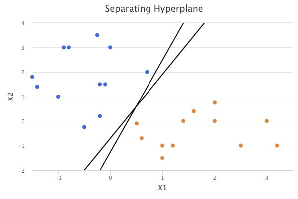
This is where the maximal margin classifier helps determine the hyperplane to use.

Maximal Margin Classifier

The maximal margin classifier is a separating hyperplane that is farthest from the training observations.

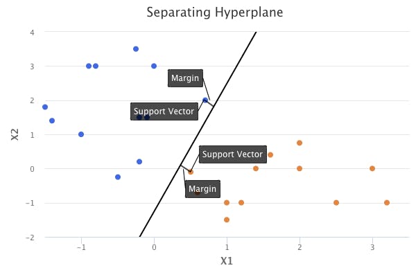
The method involves determining the perpendicular distance from each training observation to some hyperplane. The smallest such distance is known as the margin. The maximal margin classifier settles on the hyperplane for which the margin is largest. In other words, the chosen hyperplane is the one that has the farthest minimum distance to the training observations.

The maximal margin classifier is often successful, but can lead to overfitting when we have a lot of predictors in our dataset.

The points that end up supporting the maximal margin hyperplane are known as support vectors. If these points are moved even slightly, the maximal margin hyperplane would move as well. The fact that the maximal margin hyperplane depends only on a small subset of observations is an important property that will also be discussed in the sections on support vector classifiers and support vector machines.

Construction of the Maximal Margin Classifier

The maximal margin hyperplane is the solution to an optimization problem with three components:

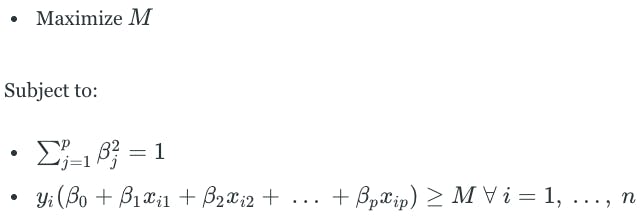
M is the margin of the hyperplane. The second component is a constraint that ensures that the perpendicular distance from any observation to the hyperplane is given by the following:

The third component guarantees that each observation will be on the correct side of the hyperplane, with some cushion M.

Non-separable Case

The maximal margin classifier is a natural way to perform classification, but only if a separating hyperplane exists. However, that is usually not the case in real-world datasets.

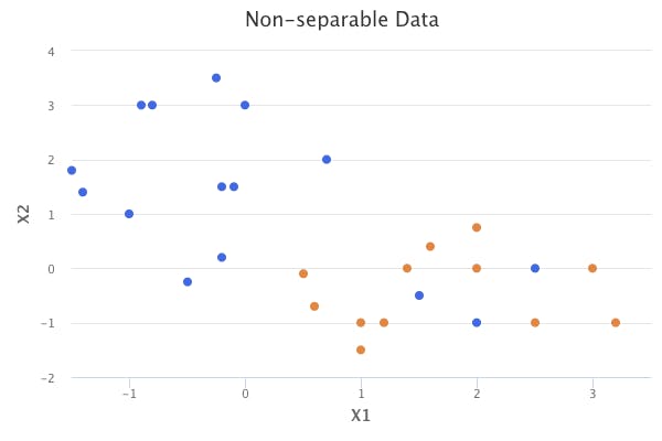
The concept of the separating hyperplane can be extended to develop a hyperplane that almost separates the classes. This is done by using a soft margin. The generalization of the maximal margin classifier to the non-separable case is known as the supper vector classifier.

Support Vector Classifier

In most cases, we usually don’t have a perfectly separating hyperplane for our datasets. However, even if we did, there are cases where it wouldn’t be desirable. This is due to sensitivity issues from individual observations. For example, the addition of a single observation could result in a dramatic change in the maximal margin hyperplane.

Therefore, it is usually a good idea to consider a hyperplane that does not perfectly separate the classes. This provides two advantages:

• Greater robustness to individual observations
• Better classification of most of the training observations

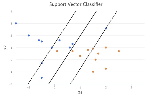
In other words, it is usually worthwhile to misclassify a few training observations in order to do a better job of classifying the other observations. This is what the support vector classifier does. It allows observations to be on the wrong side of the margin, and even the wrong side of the hyperplane.

Details of the Support Vector Classifier

The support vector classifier will classify a test observation depending on what side of the hyperplane that it lies. The hyperplane is the solution to an optimization problem that is similar to the one for the maximal margin classifier.

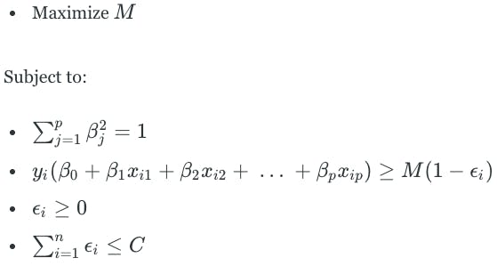
M is the margin of the hyperplane. The second component is a constraint that ensures that the perpendicular distance from any observation to the hyperplane is given by the following:

ϵ is a slack variable that allows observations to be on the wrong side of the margin or hyperplane. It tells us where the i-th observation is located, relative to the hyperplane and margin.

• If ϵ = 0, the observation is on the correct side of the margin
• If ϵ > 0, the observation is on the wrong side of the margin
• If ϵ > 1, the observation is on the wrong side of the hyperplane

C is a nonnegative tuning parameter that bounds the sum of the ϵ values. It determines the number and severity of violations to the margin and hyperplane that will be tolerated.

In other words, C is a budget for the amount that the margin can be violated by the n observations. If C = 0, then there is no budget, and the result would simply be the same as the maximal margin classifier (if a perfectly separating hyperplane exists). If C > 0, no more than C observations can be on the wrong side of the hyperplane because ϵ > 1 in those cases, and the constraint from the fourth component doesn’t allow for it. As the budget increases, more violations to the margin are tolerated, and so the margin becomes wider.

It should come as no surprise that C is usually chosen through cross-validation. C controls the bias-variance tradeoff. When C is small, the classifier is highly fit to the data, resulting in high variance. When C is large, the classifier may be too general and oversimplified for the data, resulting in high bias.

In support vector classifiers, the support vectors for the hyperplane are a bit different than the ones from the maximal margin hyperplane. They are the observations that lie directly on the margin and the wrong side of the margin. The larger the value of C, the more support vectors there will be.

The fact that the supper vector classifier is based only on a small subset of the training data means that it is robust to the behavior of observations far from the hyperplane. This is different from other classification methods such as linear discriminant analysis, where the mean of all observations within a class help determine the boundary. However, support vector classifiers are similar to logistic regression because logistic regression is not very sensitive to observations far from the decision boundary.

Support Vector Machines

First, we will discuss how a linear classifier can be converted into a non-linear classifier. Then, we’ll talk about support vector machines, which do this in an automatic way.

Classification with Non-linear Decision Boundaries

The support vector classifier is a natural approach for classification in the binary class setting, if the boundary between the classes is linear. However, there are many cases in practice where we need a non-linear boundary.

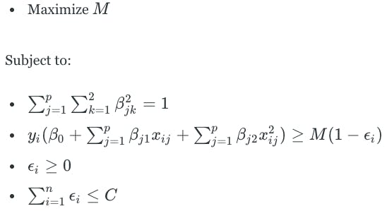
In chapter 7, we were able to extend linear regression to address non-linear relationships by enlarging the feature space by using higher-order polynomial functions, such as quadratic and cubic terms. Similarly, non-linear boundaries can be created through the use of higher-order polynomial functions. For example, we could fit a support vector classifier using each predictor and its squared term:

This would change the optimization problem to become the following:

However, the problem with enlarging the feature space is that there are many ways to do so. We could use cubic or even higher-order polynomial functions. We could add interaction terms. Many possibilities exist, which could lead to inefficiency in computation. Support vector machines allow for enlarging the feature space in a way that leads to efficient computations.

Support Vector Machines

The support vector machine is an extension of the support vector classifier that enlarges the feature space by using kernels. Before we talk about kernels, let’s discuss the solution to the support vector classifier optimization problem.

Solution to Support Vector Classifier Optimization Problem

The details of how the support vector classifier is computed is highly technical. However, it turns out that the solution only involves the inner products of the observations, instead of the observations themselves. The inner product of two vectors is illustrated as follows:

The linear support vector classifier can be represented as:

There are n parameters (αᵢ) per training observation. The parameters are estimated with the inner products between all pairs of training observations.

To evaluate the support vector classifier function f(x), we compute the inner product between a new observation x and each training observation xᵢ. However, the αᵢ parameters are nonzero only for the support vectors. In other words, if an observation is not a support vector, then its αᵢ is zero. If we represent S as the collection of the support vectors, then the solution function can be rewritten as the following:

Kernels

A kernel is a function that quantifies the similarity of two observations, and is a generalization of the inner product. The kernel function used in the support vector classifier is simply

This is known as a linear kernel because the support vector classifier results in a linear boundary. The linear kernel determines the similarity of observations by using the Pearson correlation.

Instead of using the linear kernel, we could use a polynomial kernel:

Using a nonlinear kernel results in a non-linear decision boundary. When the support vector classifier is combined with a nonlinear kernel, it results in the support vector machine. The support vector machine takes on the form:

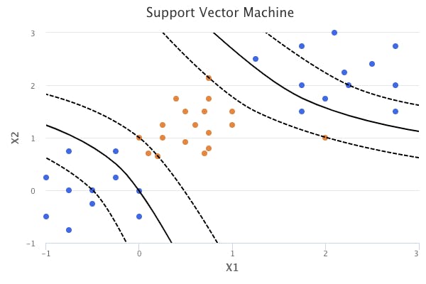
The polynomial kernel is just one example of a nonlinear kernel. Another common choice is the radial kernel, which takes the following form:

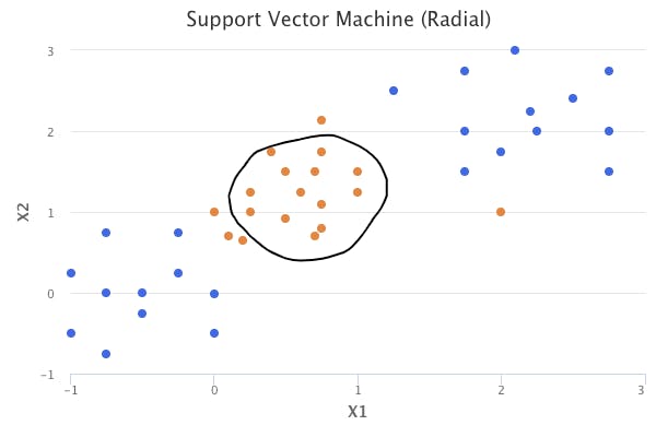
The advantage to using kernels is that the computations can be performed without explicitly working in the enlarged feature space. For example, in the polynomial kernel, we are simply determining the summation of the inner products, and then transforming our result to a higher degree or dimension d. This is known as the kernel trick.

SVMs with More than Two Classes

The concept of separating hyperplanes upon which SVMs are based does not lend itself naturally to more than two classes. However, there are a few approaches for extending SVMs beyond the binary class setting. The most common approaches are one-versus-one and one-versus-all.

One-Versus-One Classification

A one-versus-one or all-pairs approach develops multiple SVMs, each of which compares a pair of classes. Test observations are classified in each of the SVMs. In the end, we count the number of times that the test observation is assigned to each class. The class that the observation was assigned to most is the class assigned to the test observation.

One-Versus-All Classification

The one-versus-all approach develops multiple SVMs, each of which compares one class to all of the other classes. Assume that each SVM resulted in the following parameters from comparing some class k to all of the others:

Let x represent a test observation. The test observation is assigned to the class for which the following is the largest:

SVMs vs Logistic Regression

As previously mentioned, only the support vectors end up playing a role in the support vector classifier that is obtained. This is because the loss function is exactly zero for observations that are on the correct side of the margin.

The loss function for logistic regression is not exactly zero anywhere. However, it is very small for observations that are far from the decision boundary.

Due to the similarities between their loss functions, support vector classifiers and logistic regression often give similar results. However, when the classes are well separated, support vector machines tend to perform better. In cases where there is more overlap, logistic regression tends to perform better. In any case, both should always be tested, and the method that performs best should be chosen.

Originally published at https://www.bijenpatel.com on August 9, 2020.

I will be releasing the equivalent Python code for these examples soon. Subscribe to get notified!

ISLR Chapter 9 — R Code

Support Vector Classifiers

library(ISLR)
library(MASS)
library(e1071)

# We will generate a random dataset of observations belonging to 2 classes
set.seed(1)
x=matrix(rnorm(20*2), ncol=2)
y=c(rep(-1, 10), rep(1, 10))
x[y==1,]=x[y==1,] + 1

plot(x, col=(3-y))

# To use SVM, the response must be encoded as a factor variable
data = data.frame(x=x, y=as.factor(y))

# Fit a Support Vector Classifier with a cost of 10
# The scale argument is used to scale predictors
# In this example, we will not scale them
svmfit = svm(y~., data=data, kernel="linear", cost=10, scale=FALSE)

# Plot the fit
plot(svmfit, data)

# Determine which observations are the support vectors
svmfit$index

# Fit an SVM with a smaller cost of 0.1
svmfit = svm(y~., data=data, kernel="linear", cost=0.1, scale=FALSE)

# The e1071 library contains a tune function
# The function performs cross-validation with different cost values
set.seed(1)
tune.out = tune(svm, y~., data=data, kernel="linear", ranges=list(cost=c(0.001, 0.01, 0.1, 1, 5, 10)))

# Check the summary to see the error rates of the different models
# The model with a cost of 0.1 has the lowest error
summary(tune.out)

# Choose the best model
bestmod = tune.out$best.model
summary(bestmod)

# The predict function can be used to predict classes on a set of test observations
xtest = matrix(rnorm(20*2), ncol=2)
ytest = sample(c(-1, 1), 20, rep=TRUE)
xtest[ytest==1,]=xtest[ytest==1,] + 1
testdata=data.frame(x=xtest, y=as.factor(ytest))
ypred = predict(bestmod, testdata)
table(predict=ypred, truth=testdata$y)</span>

Support Vector Machines

# Now, we will fit a Support Vector Machine model
# We can do this by simply using a non-linear kernel in the svm function

# Generate a dataset with a non-linear class boundary
set.seed(1)
x=matrix(rnorm(200*2), ncol=2)
x[1:100,]=x[1:100,]+2
x[101:150,]=x[101:150,]-2
y=c(rep(1, 150), rep(2, 50))
data = data.frame(x=x, y=as.factor(y))
plot(x, col=y)

# Split the data into training and test sets
train = sample(200, 100)

# Fit an SVM with a radial kernel
svmfit=svm(y~., data=data[train,], kernel="radial", gamma=1, cost=1)
plot(svmfit, data[train,])

# Perform cross-validation using the tune function to test different choices for cost
set.seed(1)
tune.out = tune(svm, y~., data=data[train,], kernel="radial",
                ranges=list(cost=c(0.1, 1, 10, 100, 1000),
                gamma=c(0.5, 1, 2, 3, 4)))
summary(tune.out)
# Cost of 1 and Gamma of 2 has the lowest error

# Test the model on the test dataset
table(true=data[-train,"y"], pred=predict(tune.out$best.model, newx=data[-train,]))</span>